The VMworld Europe keynote featured the future VMware Cloud on AWS services. In short this services gives VMware customers instant scale and global reach delivered by AWS while continuing to use their own skill set driving and operating VMware SDDC environments on-prem and in-cloud. Avoid the risk that comes with re-platforming, re-architecting current application landscape to run on a different platform while providing the same service. In turn it allows the IT organization to connect the current applications with AWS vast service catalog and use services like RDS, Red Shift, Glacier and many more.
One of the interesting features that is under tech preview is Elastic DRS. Elastic DRS helps to solve one of the toughest challenges an IT architect can face: capacity planning. Major key points of capacity planning are current and future resource demand, failure recovery capacity and maintenance capacity. Finding the right balance between maintaining workload performance versus the downside of CAPEX and OPEX of reserved failover capacity is difficult. By leveraging the IT-at-scale operations of AWS, Elastic DRS transforms vSphere clusters into an agility powerhouse.
 
Rapid scaling ability allows to add additional hosts to the cluster. No more ordering new hardware, racking and stacking, just add the new host to the cluster with a right-click of the mouse. By using native metrics, DRS can detect that the cluster is running out of host resources and presents a recommendation of adding another host. Like regular DRS, you can also put Elastic DRS into automatic mode and allow it to add or remove hosts based on observed load on the cluster.

Sometimes we forget how extremely complex running IT at super scale is. Automating the install, configuration and operaing one host is interesting, doing this by the dozen is already pushing the limits for a lot of IT organizations. Now think about this doing it in more than a dozen datacenters around the world at the same time while being required to do it instantly when a customer wants this. Undeniably impressive. When joining the team, learning about Elastic DRS was exciting, understanding how this works for all the customers on all the AWS datacenters around the world is just mind-blowing! IT-at-Scale to its finest.
When you have ready-to-go ESXi hosts at your fingertips it allows you to do so many cool things , for example allow DRS to aid and assist vSphere HA. Since ESXi 3.0, vSphere HA has ensured that workloads are restarted on the surviving hosts in the cluster. However, when a host outage is not temporary, but permanently, application performance can be impacted due to the reduction of available host resources on a longer term. Auto remediation helps to address this challenge.
Auto remediation builds upon Elastic DRS and ensures that the available host resources remain consistent during an ESXi host outage. When a host failure is detected, auto remediation adds another hosts to the cluster, ensuring that the workload performance will not be impacted in the long run by a host failure. If partial (hardware) failure occurs, auto remediation ensures that VSAN operations complete before ejecting the degraded host.
 
Another benefit of this framework is the ability to retain similar levels of resources during maintenance. Typically during maintenance operations, hosts are patched and temporarily unavailable to run and service applications. Many IT organizations deal with this situation, by either “oversizing” cluster or by offering SLA’s that provides a reduced service during maintenance hours. With Elastic DRS, the cluster size is not reduced during maintenance operations. This way workloads are not impacted by a loss of resources and continue to perform similarly as to normal operation hours.
To emphasize this is a a technical preview of a service that is not operational yet.
For more info about VMware Cloud on AWS, take a closer look.

After a long time of keeping this silent, I can finally share a little bit what I’ve been focussing on at VMware. (This is a repost of content on blogs.vmware.com)
Today, VMware and Amazon Web Services (AWS) are announcing a strategic partnership providing the ability to run a full VMware Software Defined Data Center (SDDC) as a cloud service on AWS. This service will include all the enterprise tools you’re familiar with including vSphere, ESXi, VSAN and NSX. This article provides a technical preview of the new service VMware Cloud on AWS (VMC), allowing me to give you a sneak peak of the incredibly cool stuff that is coming.

This architecture is a match made in heaven if you ask me. It allows administrators and architects that are used to vSphere to leverage the agility of AWS without re-architecting applications and reconstructing operational procedures. One great advantage is that vCenter will be the main platform of operations, therefore all tools that you currently run against vCenter in your on-premises vSphere deployment will work with the in-cloud SDDC environment. All these tools and functionalities that have been developed over the years are now coming together and provide an environment that allows workload mobility between clouds while pushing data center agility to new levels.
In short, once signed up, select a cluster size and a SDDC environment is created for you in a very short time. To emphasize (and to avoid any misconception), the VMware cloud will run on native ESX on next-generation, bare metal AWS Infrastructure. The VMware cloud will be deployed as a private cloud containing vSphere ESXi hosts, VSAN and NSX on AWS infrastructure. This will allow you to run enterprise workloads with the same performance, reliability and availability levels as your on-premises vSphere deployments but now on an AWS architecture. The main difference between the on-prem and in-cloud deployment is that VMware manages and operates the infrastructure of the VMware Cloud on AWS.

It is important to note here that this is a fully managed service. That is to say, VMware will install, manage and maintain the underlying ESXi, VSAN, vCenter and NSX infrastructure. Routine operations like patching or hardware failure remediation will be taken care of by VMware as part of the service. Customers will have delegated permissions to things like vCenter and will be able to use vCenter to perform administrative tasks but there will be some actions like patching which VMware will provide to you as part of the service. This means that VMware takes care of the core infrastructure in partnership with AWS.
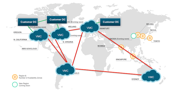
VMware Cloud on AWS will be available as a stand-alone deployment, as a Hybrid cloud deployment or as a cloud-to-cloud deployment. With hybrid and cloud-to-cloud deployments, vCenter enhanced linked-mode provides a single pane of glass that assists IT operation teams to manage the SDDC deployments from a centralized console. NSX extends this single pane of glass by providing consistent network and security services between the various deployments. However, NSX is not a requirement! If you are not running NSX on premise right now, you will still be able to run VMware Cloud on AWS but you won’t be able to utilize the hybrid cloud features of NSX until you do. With the ability to span networks and clouds, vMotion provides workload mobility, allowing the movement of workloads in and out the various cloud deployments. Yes, you read that correctly, you can vMotion from your existing on-premises vSphere environment to AWS!
One of the interesting concepts is elastic scaling. Elastic scaling would help to solve one of the toughest challenges an IT architect can face: capacity planning. Major key points of capacity planning are current and future resource demand, failure recovery capacity and maintenance capacity. Finding the right balance between maintaining workload performance versus the downside of CAPEX and OPEX of reserved failover capacity is difficult. Think about how elastic scaling would transform vSphere clusters into agile powerhouses. Instead of going through the tedious procuring and installing process yourself, benefit from the IT-at-scale mindset and services delivered by AWS.
Since ESXi 4.0, vSphere HA has enabled workloads to restart the surviving hosts in the cluster. However, when a host outage is not temporary, host resources can become constrained due to the reduction of the available hosts. Auto-remediation can builds upon DR solutions ensuring available host resources remain consistent during an ESXi host outage. When a host failure is detected, auto-remediation adds other hosts to the cluster, ensuring that the workload performance will not be impacted in the long run by a host failure. If partial (hardware) failure occurs, auto-remediation ensures that VSAN operations complete before ejecting the degraded host.
Another benefit of this framework is the ability to retain similar levels of resources during maintenance. During maintenance operations, the cluster size is not reduced, workloads are not impacted by a loss of resources and continue to perform similarly as to normal operation hours.
I believe one of the strengths of VMware Cloud on AWS service is that it allows administrators, operation teams and architects to use their existing skill set and tools to consume AWS infrastructure. You can move workloads to the cloud without having to replatform them in any way, no conversion of virtual machines, no repackaging and very important no extensive testing, you just migrate the VM. Another strength it the ability to pair current workloads with the advanced feature set of AWS. As a result, IT teams will be able to extend their skill set discovering the vast catalog of services AWS has to offer. This creates an environment that works seamlessly with both on-premises private clouds and advanced AWS Public Cloud Services.
There are so many other great features that I want to cover, but let’s save that for future articles.

VMworld

If you want to learn more about the upcoming service VMware Cloud on AWS, come join us at VMworld Europe, breakout session INF7849: VMware Cloud on AWS – a closer look. In this session Alex Jauch and I dive a little deeper into the details of this service. For a more generic view, please register for the breakout session INF7711 – VMware Cloud Foundation on Public Clouds.
At VMworld Europe, I have a limited set of Meet the expert slots available to me, please register if you would like to have a more focused conversation about the service.
If you are interested in applying for the beta, please click here: http://learn.vmware.com/37941_REG

I’m excited to announce that I’ve accepted a position at VMware as Senior Staff Architect. I can’t share the details of this next-level product that I will be working on right now. But I look forward to sharing more information when the time is right. I cannot wait to get started.
#GameOn!