Machine Learning on VMware Cloud Platform – Part 1 covered the three distinct phases: concept, training, and deployment, part 2 explored the data streams, the infrastructure components needed and vSphere can help with increasing resource utilization efficiency of ML platforms. In this part, I want to go a little bit deeper into the territory of training and inference workloads.

It would be best to consider the platform’s purpose when building an ML infrastructure. Are you building it for serving inference workloads, or are you building a training platform? Are there data science teams inside the organization that create and train the models themselves? Or will pre-trained models be acquired? Where will the trained (converged) model be deployed? Will it be in the data center, industrial sites, or retail locations?

From an IT architecture resource requirement perspective, these training and inference workloads differ in computational power and data stream requirements. One of the platform architect’s tasks is to create a platform that reduces the time to train. It’s the data scientist’s skill and knowledge to use the platform’s technology to reduce the time even more without sacrificing accuracy.

This part will dive into the key differences between training and inference workloads and their requirements. It helps you get acquainted with terminology and concepts used by data scientists and apply that knowledge to your domain of expertise. Ultimately, this overview helps set the stage for presenting an overview of the technical solutions of the vSphere platform that accelerate machine learning workloads.

Types of machine learning algorithms

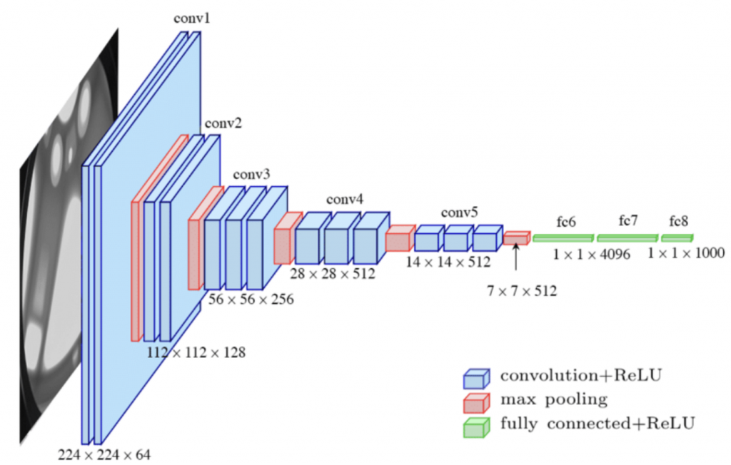
When reviewing popular machine learning outlets and podcasts, you typically only hear about training large models. For many, machine learning equals deep learning with giant models and massive networks that require endless training days. But in reality, that is not the case. We do not all work at the most prominent US bank. We do not all need to do real-time fleet management and route management of worldwide shipping companies or calculate all possible trajectories of five simultaneously incoming tornadoes. The reality is that most companies work on simple models with simple algorithms. Simple models are easier to train. Simple models are easier to test. Simple models are not resource-hogs, and above all, simple models are simpler to update and keep aligned with the rapidly changing world. As a result, not every company is deploying a deep-learning GPT-3 model or massive ResNet to solve their business needs. They are looking at “simpler” machine learning algorithms or neural networks that can help increase the revenue or decrease the business cost without running it on 400 GPUs.

In the following articles, I will cover neural networks, but if you are interested in understanding the basics of machine learning algorithms I recommend looking at the following popular ones:

Support Vector Machines (SVM)

Decision trees

Logistic Regression

Random forest

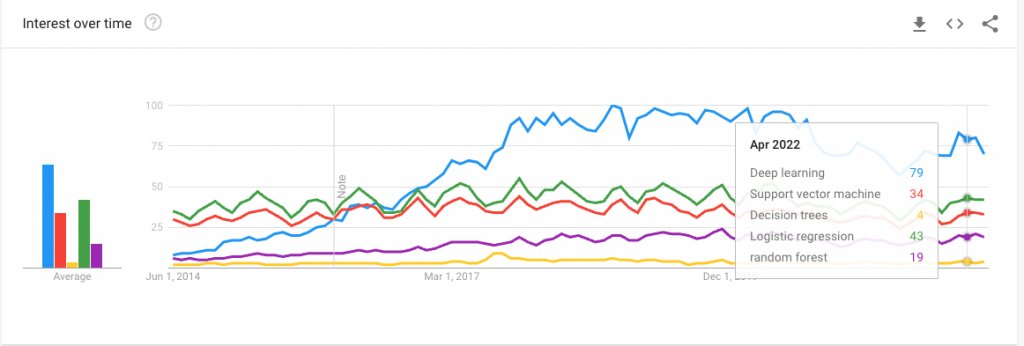
k-means (not listed in the google search result)

Data Flow

Training produces a neural network model that generates a classification, detection, recommendation, or any other service with the highest level of accuracy. The golden rule for training is that the more data you can use, the higher accuracy you achieve. That means the data scientist will unleash copious amounts of data on the system. Understanding the data flow and the components involved helps you design a platform that can significantly reduce training time.

Most neural networks are trained via the (offline) batch learning method, but the online training method is also used. In this method, the model is trained by feeding it smaller batches of data. The model is active and learns on the fly. Whether it is less resource-intensive than batch learning, or often referred to as offline training, is debatable as the model trains itself continuously. It needs to be monitored very carefully as it can be sensitive to new data that can quickly influence the model. Specific stock price systems deploy ML models that use online training to respond to market trends quickly.

The inference service is about latency, for example, pedestrian identification in autonomous vehicles, packages flying across high-speed conveyor belts, product recommendations, or speech-to-text translations. You simply cannot afford to wait on a response from the system in some cases. Most of these workloads are a single data sample or, at best, a small number of instructions batched up. The data flow of inference is considered to be streaming of nature. As a result, the overall compute load of inference is much lower than that of the training workload. 

	Training	Inference
Data Flow	Batch Data	Streaming Data

Data sets and Batches

During model training, models train with various data sets: training sets, validation sets, and testing sets. The training set helps the model recognize what it should be supposed to learn. The validation dataset is helpful for the data scientist to understand the effect of tuning particular hyperparameters, such as the number of hidden layers or the network layer size. The third dataset is the testing set and proves how well the trained neural network performs on unseen data before being put into production.

A dataset provides the samples used for training. These data sets can be created from company data or acquired from third parties. Or a combination of both, sometimes businesses acquire extra data on top of their own to get better insights into their customers. These datasets can be quite large. An example is a Resnet50 model with Imagenet-1K dataset. Resnet50 is an image classification training network, and the Imagenet-1K dataset contains 1.28 million images (155.84 GiB).

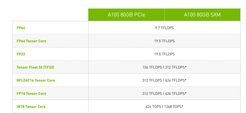
Even the latest NVIDIA GPU generations (Ampere and Hopper) offer GPU devices with up to 80GB of memory and cannot fit that dataset entirely in memory. As a result, the dataset is split into smaller batches. Batch size plays a significant role in the training of neural network models. This training technique is called mini-batch gradient descent. Besides circumventing the practical memory limitation, It impacts the accuracy of models, as well as the performance of the training process.  If you’re curious about batch sizing, read the research paper “Revisiting small batch training for deep neural networks“. Let’s cover some more nomenclature while we are at it.

During the training cycle, the neural network processes the dataset’s examples. This cycle is called an epoch. A data scientist splits up the entire dataset into smaller batch sets. The number of training examples used is called a batch size. An iteration is a complete pass of a batch. The number of iterations is how many batches are needed to complete a single epoch. For example, the Imagenet-1K dataset contains 1.28 million images. Well-recommended batch size is 32 images. It will take 1.280.000 / 32 = 40.000 iterations to complete a single epoch of the dataset. Now how fast an epoch completes depends on multiple factors. A training run typically invokes multiple epochs. 

Both training and inference use batch sizes. In most use cases, inference focuses on responding as quickly as possible. Many inference use-cases ingest and transform data in real-time and generate a prediction, classification, or recommendation. Translating this into real-life use cases, we are talking about predicting stock prices to counting cars in a drive-through. The request needs to be processed the moment it comes in. As a result, no batching to limited batching occurs. It depends on how much workload the system receives when it is operational. By batching 1-4 examples, Inference classes as streaming workload.

Determining the correct batch size for training is a science by itself. Many research papers and Medium articles exist about the sweet spot for batch sizes. There are benefits and disadvantages to be found at any point in the spectrum of batch sizes. Smaller batch sizes can lead to lower memory footprint and improvement of throughput, while larger batch sizes can increase parallelism and decrease the computational cost.

This last factor might not be relevant for a data scientist when training in an on-premises environment, but it’s good to understand. When batches are moved from storage or host memory to GPU device memory, CPU cycles are needed. If you are using larger batches, you reduce the number of computing calls to move data, ultimately reducing your CPU footprint. Off course, there is a downside to this as well, primarily on the performance side of the algorithm, something the data scientist needs to figure out how to solve. Therefore you notice that depending on the use case, you see different batch sizes per model. Two excellent papers that highlight both ends of the spectrum: “Friends don’t let friends use mini-batches larger than 32” and “Scaling TensorFlow to 300 million predictions per second“

The takeaway for the platform architect is that inference is primarily latency-focused. If the inference workload is a video-streaming-based workload for image classification or object detection, the system should be able to provide a particular level of throughput. Training is predominantly throughput based. Batch sizing is a domain-specific (hyper)parameter for the data scientist. Still, it can ultimately affect the overall CPU footprint and whether efficient distributed training is used. Depending on the dataset size, the data scientist can opt for distributed training, dispatching the batches across multiple GPUs.

	Training	Inference
Storage Characteristics	Throughput based	Latency-based, occasionally throughput
Batch Size	Many recommendations between 1-32 Smaller batch size reduces the memory footprint Smaller batch size increases algorithm performance (generalization)  Larger batch size increases compute efficiency Larger batch size increases parallelization (Multi-gpu)	1-4

Data Pipeline and Access Patterns

Data loading is essential to building a deep Learning pipeline and training a model. Remember that everything you do with data takes up memory. Let’s go over the architecture and look at all the “moving parts” before diving into each one.

The dataset is stored on a storage device. It can be a vSAN datastore or any supported network-attached storage platform (NFS, VMFS, vVOLs). The batch is retrieved from the datastore and stored in host memory before it loads into GPU device memory (Host to Device (HtoD)). Once the model algorithm completes the batch, the algorithm copies the output back to host memory (Device to Host – DtoH). Please note that I made a simple diagram and showed the most simple data flow. Typically, we have a dual-socket system, meaning there are interconnects involved, multiple PCI controllers involved, and we have to deal with VM placement regarding the NUMA locality of the GPU. But these complex topics are discussed later in another article. one step at a time.

We immediately notice the length of the path without going into the details of NUMA madness. Data scientists prefer that the dataset is stored as close to the accelerator as possible on a fast storage device. Why? Data loading can reduce the training time tremendously. Quoting Gorkem Polat, who did some research on his test environment:

One iteration of the ResNet18 Model on ImageNet data with 32 batch size takes 0.44 seconds. For 100 epochs, it takes 20 days! When we measure the timing of the functions, data loading+preprocessing takes 0.38 seconds (where 90% of this time belongs to the data loading part) while the optimization (forward+backward pass) time takes only 0.055 seconds. If the data loading time is reduced to a reasonable time, full training can be easily reduced to 2.5 days! Source

Most datasets are too large to fit into the GPU memory. Most of the time, it does not make sense to preload the entire dataset into host memory. The best practice is to prefetch multiple batches and thereby mask the latency of the network. Most ML frameworks provide built-in solutions for data loading. The data pipeline can run asynchronously with training as long as the pipeline prefetches several batches to keep it full. The trick is to keep multiple pipelines full, where fast storage and low-latency and high throughput networks come into play. According to the paper “ImageNet training in Minutes,” it takes an Nvidia M40 GPU 14 days to finish just one 90-epoch Resnet-50 training execution on the ImageNet-1k dataset. The M40 was released in 2015 and had 24GB of memory space. As a result, data scientists are looking at parallelization, distributing the workload across multiple GPUs. These multiple GPUs need to access that dataset as fast as possible, and they need to communicate with each other as well. There are multiple methods to achieve multi-GPU accelerator setups. This is a topic I happily reserve for the next part. 

Dataset Random Read Access

To add injury after insult, training batch reads are entirely random. The API lets the data scientist specify the number of samples, and that’s it. Using a Pytorch example:

train_loader = torch.utils.data.DataLoader(train_set, batch_size=32, shuffle=True, num_workers=4)

The process extracts 32 random examples from the dataset and sends them over as a batch. The command Shuffle=true is for what happens after the Epoch completes. This way, the next Epoch won’t see the same images in the same order. Extracting 32 random examples from a large dataset on a slow medium won’t help reduce the training time. Placing the dataset on a bunch of spindles would drive (pun intended) your data science team crazy. Keeping the dataset on a fast medium and possibly as close to the GPU device as possible is recommended.

	Training	Inference
Data Access	Random Access on large data set Multiple batches are prefetches to keep the pipeline full Fast storage medium recommended Fast storage and network recommended for distributed training	Streaming Data

The next part will cover the memory footprint of the model and numerical precision.

This training versus inference workload series provides platform architects and owners insights about ML workload characteristics. Instead of treating deep neural networks as black box workloads, ML architectures and techniques are covered with infrastructure experts in mind. A better comprehension of the workload opens up the dialog between infrastructure and data science teams, hopefully resulting in better matching workload requirements and platform capabilities.

Part 3 of the series focussed on the memory consumption of deep learning neural network architectures. It introduced the different types of operands (weights, activations, gradients) and how each consumes memory and requires computational power throughout the different stages and layers of the neural network. Part 4 showed that a floating point data type impacts a neural network’s memory consumption and computational power requirement. I want to cover neural network compression in this part of the training versus inference workload deep dive. The goal of neural network compression is inference optimization to either help fit and run a model at a constrained endpoint or to reduce inference infrastructure running costs.

A data science team’s goal is to create a neural network model that provides the highest level of accuracy (Performance in data science terminology). To achieve high levels of accuracy, data science teams feed high-quality data sets to the ML platform and execute multiple training runs (epochs). The ML community builds newer, more complex, and more extensive neural networks to improve precision. The chart below shows the growth of parameters of image classification (orange line) and Natural Language Processing (blue line) in state-of-the-art (SOTA) neural network architectures.

If we deconstruct any neural network architecture, we can see that each neural network has different layers and operands, i.e., weights, activations, and gradients. These layers and operands impact a model’s performance and inference time. Data scientists select an appropriate floating-point data type to reduce the neural network model’s memory utilization and increase the processing speed.

Sometimes, the neural network size (the memory footprint) prohibits successful deployment to the target production infrastructure. For example, it can be an edge deployment onto a particular device, a physical space with a restricted-energy envelope. As a result, the data science team can optimize the network even further by performing quantization. Post-training quantization converts floating point data points into integers. If done smartly, it can reduce the neural network memory footprint tremendously while retaining accuracy. An additional technique to improve the efficiency of the algorithm is pruning. Pruning and quantization go hand in hand. The CERN Large Hadron Collider team is exploring a Quantization-Aware Pruning technique.

Pruning

Pruning helps to identify the important connections within the neural network and uses methods to remove either the connection to individual weights (unstructured pruning) or remove the connection of groups of weights by disconnecting an entire channel or filter (structured pruning). The most popular frameworks, like TensorFlow (Keras) and Pytorch, contain standard modules to perform unstructured pruning on neural networks. 

An interesting thing about pruning is that many online literature and research papers use the terms remove or delete weights. It does not change the neural network layout. See the screenshot of the Optimal Brain Damage research paper, or check out the PyTorch Pruning tutorial.

When replacing the trained parameter with a zero, sparsity is introduced into the tensor or dense matrix data structure. Sparsity is the proportion of zero to non-zero weights. Algorithms can use sparsity to speed up or compress the footprint of the neural network.  

Pruning is possible as many weights in a trained neural network end up close to the value of zero. Many researchers believe that most neural networks are over-parameterized. As a result, pruning has been a hot topic since the 90s. There have been some influential papers that are still referenced today and used as the starting point for research on new pruning techniques:

In the paper “Optimal Brain Damage,” LeCun et al. discover that “reducing the size of a learning network” improved generalization (the neural network’s ability to adapt correctly to new, previously unseen data) and inference speed.  

Fast forward to 2015, Han et al. published “deep compression,” combining pruning, trained quantization, and Huffman coding to reduce the neural network footprint for mobile and other low-power applications. The pruning mechanism is (unstructured) magnitude-based, the most common today. Magnitude-based pruning assumes that the weight with the smallest value has the most negligible contribution to the neural network’s performance and removes those weights. 

Interestingly, if you train a network and prune the network connections, you end up with a neural network that retains its accuracy but has more than 50% of fewer parameters. However, if you start training with that neural network architecture, it will not achieve that high accuracy level. 

In the paper “The Lottery Ticket Hypothesis: Finding Sparse, Trainable Neural Networks” (2019), Jonathan Frankle and Michael Carbin asked why training a network with the topology of the pruned network yields worse performance. They conclude that within an extensive neural network, a smaller neural network exists that would match the performance of the larger one. This “winning lottery ticket” subnetwork exists, but you can only discover it if the same weight initializations are used as the original networks. And therefore, it’s almost impossible to discover that smaller network before you train the larger one to completion. 

The paper hypothesis automatically makes you wonder as a platform operator/architect about the approach data scientists use to optimize their models. Why not start training with a small neural network and slowly build more extensive networks? (constructive approach). Getting a neural network to react to new data correctly (generalize) with a few parameters is complicated. There seems to be no traction in the research space to investigate “Constructive neural network learning” thoroughly.

Pruning Scheduling

Generally, the data science team takes a destructive approach to model development. Multiple epochs are used to train the complete neural network with all its parameters to achieve the highest accuracy possible. The next step is to apply a pruning method in which learned parameters are set to zero, and the connections are stripped away. 

The most popular pruning method is “train, prune and fine-tune.” Pruning takes place after training. The data science team determines a pruning percentage. The pruning percentage indicates the number of learned parameters that will be set to zero across the neural network. Once the pruning is complete, the neural network retrains to “recover from the loss of parameters ” these two steps are one iteration. Please keep in mind that one iteration can contain multiple epochs of training.

The data science team can choose to execute the pruning method in different ways that affect the time the accelerators are in use and when they are idling. There are two mainstream methods that I want to highlight:

• One-shot Pruning
• Iterative Pruning

One-shot pruning prunes the neural network to a target sparsity level in one iteration. The deep compression paper showed that pruning and retraining are repeated iteratively until the target sparsity threshold is met, typically resulting in higher accuracy than one-shot pruning. It’s common to prune 20% of the weights with the lowest magnitudes during one iteration. 

Generally, iterative pruning is computationally intensive and time-consuming, especially if the global target sparsity is high and the number of parameters removed at each iteration is low. The pruning extends the use of accelerator time, but downtime occurs between iteration sessions. It can be a very “jerky” process from an accelerator utilization perspective. The iterative process introduces additional criteria besides the pruning strength:

• Pruning Strength: How many weights should be removed?
• Saliency: Which weights should be pruned?
• Pruning Stop Condition: When should the pruning process end?

Commonly, the data science team evaluates the progress between iterations. During this time, the accelerator is typically assigned to a workload construct (VM, container), yet it is not productive. When reviewing accelerator use for pruning purposes, it’s not uncommon to see the same number of epochs used for training. The paper “Retrain or Not Retrain? – Efficient Pruning Methods of Deep CNN Networks” shows a great example: 

Retraining of the pre-trained Resnet50 with global sparsity of 20%. Retraining starts at epoch 104. Top5 is marked in blue, and Top1 in red. 

Sparsity

Introducing sparsity allows for efficient compression. There is the machine learning definition of compression (i.e., sparsity) and the definition we have used since Robert Jung blessed us with ARJ in MS-DOS and when Winzip burst onto the scene in 1991. Let’s use the old-school definition for now. A pruned neural network is highly susceptible to efficient compression, as you have millions of zeroes floating around. Compression is perfect if you want to reduce the model file size for the model’s distribution to mobile devices. Mobile devices have limited memory, and as the data compression paper points out, there is a power consumption difference between data retrieval from cache or SRAM. But for large retail organizations or Telco companies dealing with countless edge locations, reducing the model size can significantly speed up the distribution of the model.

But pruning is not easy, and pruning will not automatically guarantee success. Results vary widely, depending on the neural network type and task. Some architecture responds better to pruning than others. And then, of course, there is the hardware. Replacing a trained weight for a zero doesn’t make it easier for the hardware. We, as humans, know that when we multiply by zero, the answer is … zero, and any number added to 0 is equal to itself. So we take shortcuts, but this calculation needs to be executed for a computer. It cannot be ignored unless we include this logic in an algorithm.

The focus for pruning is to retain similar accuracy while increasing sparsity. However, feeding a dense matrix data structure riddled with zeroes can cause irregular memory access patterns for accelerators. And so, a sparse, dense matrix data structure isn’t always faster. The data science team has to apply more optimizations or choose structured pruning to speed up successfully on particular accelerator devices. But removing entire filters or layers dramatically changes the neural network structure’s layout and reduces the neural network accuracy. 

Hardware vendors have also been researching this field for years, especially NVIDIA. The papers “Learning both weights and connections for efficient neural networks” and “Exploring the granularity of sparsity in convolutional neural networks” by Jeff Pool et al. (Senior Architect NVIDIA) are interesting reads. With the Ampere Architecture, NVIDIA introduced sparse tensor cores and Automatic Sparsity (ASP), a concept to generate the correct sparsity level for the hardware to accelerate. 

NVIDIA Sparsity Support

Part 5 – Numerical Precision showed the spec sheet of an NVIDIA A100 (Ampere architecture), listed 624 TOPS for INT8 operations, and listed 1248 TOPS with an asterisk. Those 1248 TOPS are sparse tensor core operations following the 2:4 structured-sparse matrix pattern prescribed by NVIDIA.

This predefined pattern means any pruned neural network can get the best performance from an Ampere accelerator (A2, A30, A40, A100). It has to follow the 2:4 structured-sparse matrix pattern. And that means that two values out of each contiguous block of four must be zeroed out. In the end, 50% of the trained values across the network are replaced by a zero. This method’s beauty is that it uses metadata to track where those zeroes are stored. To some, this sounds like a sparse matrix data structure format. But the problem is that many machine learning libraries do not offer support for sparse matrices. 

So NVIDIA uses a compressed format of a dense matrix data structure which contains the trained weights and a metadata structure that is necessary for sparse tensor cores to exploit the sparsity. This format is fed into the sparse tensor cores to get that speed up. Thus from an infrastructure perspective, you need to have your development/inference infrastructure in lockstep. They have to run both the Ampere architecture. Possibly A100 for training and pruning with ASP operations, A2 accelerator cards for inference operations.

A 2:4 structured sparse matrix W and its compressed representation (source NVIDIA)

The smart part is in the metadata. The metadata stores the positions of the non-zero weights in the compressed matrix. We must look at a standard General Matrix Multiplication operation (GEMM). In a forward propagation operation, you have a matrix (A) with weights, A matrix with activations (B), and you capture the output in Matrix C. Matrix A and B are identical in dimensions for mapping the weights and activations.

What happens with the sparse operation of the Ampere architecture? The non-zero weights are in matrix A. This one is now in a compressed state, so the dimensions do not match matrix B anymore. It only needs to pull the values from the other matrix to perform the sparse operation. It needs to perform the multiplication with the trained weight. The metadata allows the algorithm to do that. As matrix A only contains non-zero values, the metadata helps the algorithm to know precisely which activation to pull from B to match up with the train values within the compressed matrix A. 

What’s next for Pruning?

NVIDIA is looking into incorporating ASP into training operations, and I can imagine this will be a significant unique selling point. As of this point, data scientists use a huge budget to train the model before starting the activities to optimize the neural network for edge deployment. These activities are not always successful. Pruning requires long fine-tuning times that could exceed the original training time by a factor of 3 or sometimes even more. Pruning consumes tremendous amounts of resources, whether on-prem or OPEX, without proper guarantees. NVIDIA has proven that sparsity can be leveraged, it is just a matter of time before other solutions pop up.

Part 4 focused on the memory consumption of a CNN and revealed that neural networks require parameter data (weights) and input data (activations) to generate the computations. Most machine learning is linear algebra at its core; therefore, training and inference rely heavily on the arithmetic capabilities of the platform. By default, neural network architectures use the single-precision floating-point data type for numerical representation. However, modern CPUs and GPUs support various floating-point data types, which can significantly impact memory consumption or arithmetic bandwidth requirements, leading to a smaller footprint for inference (production placement) and reduced training time.

Let’s look at a spec sheet of a modern data center GPU. Let’s use the NVIDIA A100 as an example. I’m aware that NVIDIA announced the Hopper architecture, but as they are not out in the wild, let’s stick with what we can use in our systems today.

This overview shows six floating-point data types and one integer data type (INT8). Integer data types are another helpful data type to optimize inference workloads, and this topic is covered later. Some floating-point data types have values listed with an asterisk. Sparsity functionality support allows the A100 to obtain these performance numbers, and sparsity is a topic saved for a future article. 

What do these numbers mean? We have to look at the anatomy of the different floating-point data types to understand the performance benefit of each one better. 

Anatomy of a Floating-Point Data Type

A fantastic 11-minute video on YouTube describes how floating-point works very well. I’ll stick to the basics that help frame the difference between the floating-point data types. The floating-point format is the standard way to represent real numbers on a computer. However, the binary system cannot represent some values accurately. Due to the limited number of bits used, it cannot store numbers with infinite precision; thus, there will always be a trade-off between range and precision. A wide range of numbers is necessary for neural network training for the weights, activations (forward pass), and gradients (backpropagation). Weights typically have values hovering around one, activations are magnitudes larger than one, and gradients are again smaller than one. Precision provides the same level of accuracy across the different magnitudes of values. 

Different floating standards exist, each with different configurations to provide range and precision. The floating-point format uses several bits to specify the decimal point placement. The floating-point bit range consists of three parts, the sign, the exponent, and the significand precision (sometimes called the mantissa). The sign bit tells us whether the value is positive or negative. The exponent part in the floating-point number tells the system where to place the decimal point. The significand precision part represents the actual digits of the number. Modern GPU specs list the following three IEEE 754-2008 standards; 

Double precision (FP64) consumes 64 bits. 1 bit for the sign value, 11 bits for the exponent, and 52 for the significand precision. 

Single precision (FP32) consumes 32 bits. 1 bit for the sign value, 8 bits for the exponent, and 23 bits for the significand precision.

Half precision (FP16) consumes 16 bits. 1 bit for the sign value, 5 bits for the exponent, and 10 for the significand precision. 

Let’s place these floating points data types in the context of deep learning. FP64 is typically not used in neural network computations as these do not require that high precision. High-Performance Computing (HPC) simulations use FP64. When reviewing GPU specs, FP64 performance shouldn’t be your first concern if you build an ML-only platform.

Single precision is the gold standard for training. Weights, activations, and gradients in neural networks are represented in FP32 by default. But much research showed that for deep learning use cases, you don’t need all that precision FP32 offers, and you rarely need all that much magnitude either. When using FP16 for training, memory requirements are reduced by fifty percent. Fewer bits to process means fewer computations are required, so the training time should be significantly faster. 

But unfortunately, there are some drawbacks. First of all, you cannot easily use FP16. It’s not a drop-in replacement code. The data scientist has to make many changes to the model to use FP16. The range offered by FP16 is significantly smaller than FP32 and can introduce two conditions during training. An underflow condition where the number moves toward zero, and as a result, the neural network does not learn anything or the overflow condition where the number becomes so large that it learns nothing meaningful. As you can imagine, underflow and overflow conditions are something data scientists always want to avoid.

But the concept of reducing memory consumption is alluring. The industry started to work on alternatives. One alternative that is now widely supported by CPU and GPU vendors is BFLOAT16.

BFLOAT16: Google Brain developed Brain Floating Point (BF16) specifically to reduce the memory consumption requirements of neural networks and increase the computation speeds of the ML algorithms. It consumes 16 bits of memory, 8 bits for the exponent, and 7 for the precision. For more information about BFLOAT16, see A Study of BFLOAT16 for Deep Learning Training. BF16 provides the same range of values as FP32, so the conversion to and from FP32 is simple. FP32 is the default data type for deep learning frameworks such as Pytorch and TensorFlow. 

Google explains the advantages of BFLOAT16 in one of their blogs:

The physical size of a hardware multiplier scales with the square of the mantissa width. With fewer mantissa bits than FP16, the bfloat16 multipliers are about half the size in silicon of a typical FP16 multiplier, and they are eight times smaller than an FP32 multiplier!

The quote tells us that the BF16 workload with seven precision bits takes half the silicon area compared to the FP16 workload that uses ten precision bits. If you compare BF16 to FP32, you can do with a system that has an eight times smaller silicon area. For Google, which designs its own ML accelerator hardware (TPU) and runs its own ML services on top of it, reducing its workload footprint is a tremendous cost saver and a service enabler. 

BF16 is more or less a truncated version of FP32, and with minimal code conversion, it can replace FP32 code. It does not require techniques such as loss scaling, which attempts to solve the underflow problem occurring with FP16, reducing boat-loads of the data scientists’ headaches. On top of that, BF16 allows the data scientist to train deeper and wider neural network models. Fewer bits to move means fewer throughput requirements, and fewer bits to compute means less arithmetic complexity, meaning less silicon area required per experiment. As a result, BF16 allows data scientist to increase their batch size or create more extensive neural networks. BF16 is becoming a prevalent floating point data type within the data science community. Look for hardware that supports the BF16 data type, such as the NVIDIA Ampere generation (A100/A30/A40/A2), AMD Instinct MI200 Accelerator GPU series, Intel Xeon Scalable Processor Third Gen supports it (Intel Deep Learning Boost AVX-512_BF16 Extension), and ARMv8-A.

From a platform operator perspective, BF16 allows more teams to use the same hardware when developing models and running experiments. As 8 GB of memory suddenly feels more like 16 GB by using lower precision, data science teams can use fractional GPUs without experiencing performance impact. That additional headroom works in favor of workload consolidation for ML workloads. Part 1 described the ML model development lifecycle, and if data science teams are currently developing models (concept phase), they can share a single GPU without drastically impacting their performance. Combine fractional GPU functionality such as NVIDIA vGPU (MIG) with a platform such as Kubernetes. You can easily create a platform that quickly attaches and detaches accelerator resources to data science teams developing new neural network models or ML-infused services. Justin Murray and Catherine Xu wrote an extensive article on deploying an AI-ready platform with vSphere and Kubernetes. Another article in this series will dive into the spectrum of ML accelerators and when to deploy fractional GPUs regarding the ML model development lifecycle. 

TensorFloat32: NVIDIA developed TensorFloat32 (TF32). TF32 is internal to CUDA, meaning only NVIDIA devices support it. This one is interesting as it’s not explicitly called in frameworks like TensorFlow or PyTorch like all the other floating point data types. Well, it’s a Tensor core mode, not a data type.

For example, if you want to use the data type BF16, you use  tf.bfloat16 in Tensorflow or torch.bfloat16 in Pytorch. With TF32, you keep using the default (FP32), tf.float32, and torch.cuda.FloatTensor (default PyTorch GPU float) and the CUDA compiler handles the conversion. 

You quickly spot the similarities when comparing TF32 to the other data types. TF32 uses the same 8-bit exponent as FP32, thus supporting the same extensive numeric range. It uses the same number of bits as FP16 for precision. As research has proved, not all 23-bits are required for ML workloads. I’ve seen some worrisome threads on hacker news and StackOverflow where people are destroying each other why it’s not called TF19, as it’s using 19-bits, so I’m not going near this topic. Let’s understand the marketing aspects of things here and that it can be a drop-in replacement of FP32. Please do not start a war in the comments section on this.

Let’s compare the performance between FP32, BF16, and TF32 of the A100 GPU listed above, and of course, these are peak performances. If the model uses FP32, the device can provide a theoretical performance of 19.5 teraFLOPS. 19.5 trillion floating-point operations per second! If the data scientists call some additional CUDA libraries, it can exploit Tensor Cores to drive up the theoretical speed to 156 teraFLOPS. To put this into perspective, this device could have run Skynet as it processed information at ninety teraflops. They just needed to use TF32. 😉 If the data scientist adjusts the framework code and uses BF16, the GPU produces 312 teraFLOPS, more speeds, but more work for the data scientist. 

TF32 is the default math mode for single precision for A100 accelerators using the NVIDIA optimized deep learning framework containers for TensorFlow, Pytorch, and MXNet. TF32 is enabled by default for A100 in framework repositories starting with PyTorch 1.7, TensorFlow 2.4, and MXNet 1.8. As a result, the data scientist must make an extra effort to avoid using TF32 when running up-to-date frameworks on an A100. That means FP32 performance specs are not necessarily the primary performance spec to look at when reviewing the accelerator’s performance. 

What sets TF32 math mode apart from the FP data types is that it converts computation operations, but all the storage of the bits remains in FP32. As a result, TF32 is only increasing math throughput but not decreasing memory bandwidth pressure like FP16 and BF16 do. And this can be hard to wrap your head around. In another article in this series, I will cover this and the concept of arithmetic intensity. I will look at a CNN’s specific operations to understand whether memory bandwidth or computational capabilities limit their performance. 

Mixed Precision: Not a floating point data type but a method. Why not combine the best of both worlds? Mixed precision training uses a combination of FP16 and FP32 to reduce the memory and math bandwidth. Mixed precision starts by keeping a copy of all the network weights in FP32. Forward pass and backpropagation pass parameters are stored in the FP16 data type. Therefore, most operations require less memory bandwidth, speeding up data transfers and increasing the math operation speeds due to lower precision. As mixed precision leans heavily on FP16, underflow and overflow can occur. Frameworks such as Tensorflow dynamically determine the loss scale if the mixed precision policy is active. If your data science teams are talking about (automatic) Mixed Precision training, pay attention to the FP16 performance claims of a GPU spec sheet, as most of the training is done with that data type.

Quantization

So far, I have mainly focused on floating-point data types in the training context. For inference, optimizing the neural network footprint may be even more critical. If the model runs in the cloud, you want to minimize infrastructure costs. If you run the model near or at the edge, hardware limitations are your primary constraint. 

Data scientists, or in some organizations, MLOps teams spend much time reducing memory footprint and the computational complexity of models before they deploy them in production. They do this by quantizing the model. 

Model quantization replaces the floating points inside the neural network with integers. This process approximates the values within the network, and due to this, accuracy loss occurs (performance). The most popular integer used is the 8-bit signed integer (INT8). You can imagine that going from capturing values in 32-bit data types to now using 8-bit values might require work to keep the network performing accurately. Song Han, Huizi Mao, and William J Dally used quantization and other optimization techniques to reduce the storage requirement of their neural networks by 35× to 49× without affecting their accuracy.

The AVX-512 instruction set includes the INT8 data type. And with each new CPU generation, they introduce improvements to the Intel Deep Learning Boost kit. In the 2nd generation scalable Xeon family, they reduced INT8 operations to a single instruction. There are rumors that Intel is removing it from the desktop CPU. I guess they want to drive the ML-related workload towards the data center CPU, forgetting that most data scientist do their concept work on laptops and workstations that don’t have Xeons. The Intel Sapphire Rapids generation will introduce a new ML suite called the Advanced Matrix Extension (AMX). If you want to dive in deep, Intel published its Intel Architecture.

Instruction Set Extensions and Future Features Programming Reference online. Chapter 3 contains all the details. Have fun! To some, it may surprise that Intel focuses on ML extensions in their CPUs, but much inference at the edge runs on them. 

As Part 4 shows, the Inference workload is, on average, a streaming workload. We now have to deal with a tiny workload that we must quickly process. GPUs are throughput and parallel beasts, and CPUs are latency-focused sprinters. We now have a choice, should we allow the CPU to process this data directly, or should we get the data through the system, from the CPU and memory, across the PCIe bus, to a GPU core that runs on a lower clock cycle than a CPU. Because there isn’t much data, we are losing the advantage of parallelism. Letting the CPU take care of that workload with the proper optimization sometimes makes more sense. A great example of the power of quantization is the story of Roblox, which uses CPUs to run its inference workload. They serve over 1 billion requests a day using a fine-tuned Bert model. 

But not every inference workload can just run on a CPU. Plenty of inference workloads generate a data stream that overwhelms a CPU. The data scientist can use a roofline analysis to determine the CPU and GPU performance headroom. Another article in this series will cover the roofline analysis. The Tesla P4 started the support for the INT8 data type, and you can imagine that the ML community hasn’t stopped looking for finding ways to optimize. Turing Architecture introduced support for INT4 precision. CPUs do not have native INT4 support. 

Hopefully, the spec sheets of GPUs will make more sense now. During conversations with the data science teams within your organization, you can translate their functional requirements to technical impact. As always, leave feedback and comments below on which topics you want to see covered in future articles.

	Training	Inference
Numerical Precision	Higher Precision Required	Lower Precision Required
Data Type	FP32	BF16
	BF16	INT8
	Mixed Precision (FP16+FP32)	INT4 (Not seen Often)

Previous parts in the Machine Learning on the VMware Platform series

• Part 1 – covering ML development lifecycle and the data science team
• Part 2 – covering Resource Utilization Efficiency
• Part 3 – Training vs Inference – Data flow, Data sets & Batches, Dataset Random Read Access
• Part 4 – Training vs Inference – Memory Consumption by Neural Networks

This article dives deeper into the memory consumption of deep learning neural network architectures. What exactly happens when an input is presented to a neural network, and why do data scientists mainly struggle with out-of-memory errors? Besides Natural Language Processing (NLP), computer vision is one of the most popular applications of deep learning networks. Most of us use a form of computer vision daily. For example, we use it to unlock our phones using facial recognition or exit parking structures smoothly using license plate recognition. It’s used to assist with your medical diagnosis. Or, to end this paragraph with a happy note, find all the pictures of your dog on your phone. 

Plenty of content discusses using image classification to distinguish cats from dogs in a picture, but let’s look beyond the scope of pet projects. Many organizations are looking for ways to increase revenue or decrease costs by applying image classification, object identification, edge perception, or pattern discovery to their business processes. You can expect an application on your platform that incorporates such functionality.

Part 3 of this series covered batch sizes and mentioned a batch size of 32, which seems a small number nowadays. An uncompressed 8K image (7680 x 4320) consumes 265 MB. The memory capacity of a modern data center GPU ranges from 16 GB to 80 GB. You would argue that it could easily fit more than 32 uncompressed (8 GB) 8K images, let alone 32 8K jpegs (896 MB). Why do we see so many questions about memory consumption on data science forums? Why are the most commonly used datasets and neural networks focused on images with dimensions hovering around the 224 x 224 image size?

Memory consumption of neural networks depends on many factors. Such as which network architecture is used and its depth. The image size and the batch size. And whether it’s performing a training operation or an inference operation. This article is by no means an in-depth course on neural networks. I recommend you follow Stanfords’ CS231n or sign up for the free online courses at fast.ai. Let’s dig into neural networks a little bit, explore the constructs of a neural network and its components and figure out why an image eats up a hefty chunk of memory. 

Understanding the workload characteristics helps with resource management, troubleshooting, and capacity planning. When I cover fractional vGPU and multi-GPU in a later part of this series, you can map these functional requirements easier to the technical capabilities of your platform. So let’s start slowly by peeling off the first layer of the onion and look at a commonly used neural network architecture for image classification, the convolutional neural network.

Convolutional Neural Networks

Convolutional neural networks (CNN) efficiently recognize and capture patterns and objects in images and are the key components in computer vision tasks. A CNN is a multilayer neural network and consists of three different types of layers. The convolution layer, the pooling layer, and the fully connected layer. The first part of the neural network is responsible for feature extraction and consists of convolution and pooling layers. I’ll cover what that exactly is in the convolution layer paragraph. The second part of the network consists of the fully connected layers and a softmax layer. This part is responsible for the classification of the image.

Convolution layer

Convolution layers are the backbone of the CNN as they perform the feature extraction. A feature can be an edge of a (license plate) number or an outline of a supermarket item. Feature extraction is deconstructing the image into details, and the deeper you go into the network, the more detailed the feature becomes. 

CNNs process an image, but how does a computer see an image? To a computer, images are just numbers. A color image, i.e., an RGB image, has a value for each red, green, and blue channel, and this pixel representation becomes the foundation for the classification pipeline.

For (us) non-native English speakers, convolution (layer) is not to be confused with convolute (make an argument complex). In the convolution layer, there is a convolve action, which means “to combine” or how something is modified by another element. In this case, the convolution layer performs a dot product between two matrices to generate a feature map containing activations. Don’t be afraid. It’s not going to be a linear algebra lesson. (I wouldn’t be able to, even if I tried). But we need to look at the convolution process and its components at a high level to better understand the memory consumption throughout the pipeline within the neural network.

A neural network is a pipeline, meaning that the process’s output is the input of the following process. There are three components in a convolution layer, an array of input, a filter, and an array of output. The initial input of a CNN is an image and is the input array(a matrix of values). The convolution layer applies a feature detector known as a kernel or filter, and the most straightforward way of describing this is a sliding window. This sliding window, also in a matrix shape, includes the neural network’s weights. Weights are learnable parameters in the neural network that are adjusted during training. The weight starts with a random value, and as training continues, it, alongside the bias (another parameter), is adjusted towards a value that provides the accurate output. The weights and biases need to be stored in memory during training and are the core IP of a trained network. Typically a CNN uses a standard kernel (filter) height and width size that determines the number of weights applied per filter. The typical kernel size is 3 x 3. This filter is applied to the input array in the case of the first convolutional layer, the image. As mentioned, the convolution layer performs a dot product between two matrices to generate a feature map containing activations. Let’s look at the image to get a better understanding.

For this example, a 3×3 filter is applied to a 6 x 6 image (normally, the image dimensions would be 224 x 224). This kernel or filter size is sometimes called the receptive field. During this process, the filter calculates a single value, called activation, by multiplying the value in the kernel with every value in the highlight input array field and then adding up the “products” to get the final output value, the activation. Output = (1*1)+(2*4)+(1*1)+(4*1)+(2*3)+(1*5)+(0*9)+(1*1)+(1*3)=1+8+1+4+6+5+0+1+3=29.

Once the activation is calculated, the filter moves over a number of pixels, determined by the stride setting. Typically this is 1 or 2 pixels. And repeats the process. Once the entire input array is processed, the output array is completed. And a new filter is applied to the input array. This output array is known as a feature map or sometimes an activation map. 

Each convolution layer has a predefined number of filters, each with a different configuration of weights. Each filter creates its own feature map, which turns into the input for the following convolutional or pooling layer. One bias parameter is applied per filter. The parameter paragraph clarifies the impact of these relationships on memory consumption. 

Pooling Layer

A pooling layer follows multiple convolution layers. It summarizes essential parts of the previous layers without losing critical information. An example is using a filter to detect the outlines of a ketchup bottle and then using the pooling layer to obscure the exact location of the ketchup bottle. Knowing the location of the bottle in a particular stage of the network is unnecessary. Therefore, a pooling layer filters out unnecessary details and keeps the network focused on the most prominent features. One of the reasons to introduce the pooling layer is to reduce as many parameters throughout the network to reduce the complexity and the computational load. To consolidate the previous feature map, it either uses an average of the numbers in a specific region (average pooling) or the maximum value detected in a specific region (max pooling). Similar to the filter applied to the input, the size is much smaller (2 x 2), and the movement (stride) is much larger (2 pixels). As a result, the size of each feature map is reduced by a factor of two., i.e., each dimension halves. 

The number of feature maps remains the same as in the previous layer.

An important detail is that there are no weights or biases present in this layer, and as a result, it’s a non-trainable layer. It’s an operation rather than a learning function of the network. It impacts the layer’s overall memory consumption, which we shall discover in a later paragraph. 

Fully Connected Layer

The fully connected layer is the poster child of neural networks. Look up any image or icon of a neural network, and you will get an artist’s impression of a fully connected layer. The fully connected layer contains a set of neurons (placeholder for a mathematical function) connected to each neuron in the following layer. 

It’s the task of the fully connected layer to perform image classification. Throughout the pipeline of convolutional layers, the filters detect specific features of the image and do not “see” the total picture. They detect certain features, and it’s the task of the fully connected layers to tie it all together. The first fully connected layer takes the feature maps of the last pooling layer and flattens the matrix into a single vector. It feeds the inputs into the neurons in its layer and applies weights to predict the correct label.

Parameters Memory Consumption

What is fascinating for us is the number of parameters involved as they consume memory. Each network architecture differs in layout and its number of parameters. There are several different CNN architectures, AlexNet (2012), GoogLeNet (2014), VGG (2014), and ResNet (2017). Today ResNet and VGG-16 are the most popular CNN architectures, often pitted against each other to find the most accurate architecture comparing training from scratch versus transfer learning. ResNet-50 vs VGG-19 vs training from scratch: A comparative analysis of the segmentation and classification of Pneumonia from chest X-ray images is a fascinating read.

Let’s use the VGG-16 neural network architecture as our example CNN to understand memory consumption better. VGG-16 is a well-documented network, so if you doubt my calculations, you can easily verify them elsewhere. VGG-16 has thirteen convolutional layers, five Max Pooling layers, and three fully-connected layers. If you count all the layers, you will see it sums up to 21, but the 16 in VGG-16 refers to the 16 layers with learnable parameters. The picture below shows the commonly used diagram illustrating the neural network configuration.

It’s important to note that memory consumption predominantly spits into two significant categories memory used to store parameters (weights & biases) and memory stored for the activations in the feature maps. The feature map memory consumption depends on the image’s height, the image’s width, and the batch’s size. The parameters’ memory remains constant regardless of the image or batch size. Let’s look at the parameters of memory consumption of the neural network first.

The VGG-16 network accepts images with a dimension of 224 x 224 in RGB. That means that there are three channels for input. The dimension of the image is not relevant in this stage for memory calculation. The first convolutional layer applies 64 filters (stated on the architectural diagram as 224 x 224 x 64). It applies a filter with a kernel size of 3 x 3, and thus we calculate 64 distinct filters applying a kernel of 3 x 3 (9) weights on three input arrays (Red channel, Blue channel, Green channel). The number of weights applied in this layer is 1,728. One bias is applied per filter, increasing the total to 1,792 parameters for this convolutional layer. Each weight is stored in memory as a float (floating point numbers), and each single-precision floating-point (FP32) occupies 4 bytes, resulting in a memory footprint of 7KB. The following article of this series covers the impact of floating point types on memory consumption.

The second layer uses the 64 feature maps produced by the first convolutional layer (CL) as input. It maintains using a 3 x 3 kernel and using 64 filters. The calculation turns into 64 inputs x 64 distinct filters using nine weights; each equals 36.864 weights + 64 biases = 36928 parameters x 4 bytes = 147 kb. 

The pooling layer applies a max pooling operation with a kernel size of 2 x 2 and a stride of 2. In essence, it is reducing the matrix size of the last feature map in half. The exact number of feature maps remain, and they act as input for the next convolutional layer as no weight is involved. No, there is no memory footprint consumed from a parameter perspective.

7kb and 147kb are certainly not earth-shattering numbers, but now let’s see the rest of the network. As you can see, the memory parameters slowly grow throughout the convolutional layers of the network and then dramatically explode at the fully connected layers. What’s interesting to note is that there is a flattening operation after the last pool layer of the feature extraction part of the network. This operation will flatten the pooled feature map into a single column that produces a long vector of input data that can pass through the fully connected layers. The 512 matrices of 7 x 7 turn into a single vector containing 25,088 activations. (Click on the image to enlarge).

In total, the network requires 540 MB to store the weights and the biases. That’s quite a footprint if you consider deploying this to edge devices. But there are always bigger fish. The state-of-the-art (SOTA) neural network for generating text GPT-3, or the third generation Generative Pre-trained Transformer, has 175 billion parameters. If we use a single-precision floating-point (FP32), it needs 700 GB of memory. Most companies don’t use a GPT-3 model to enhance their business processes, but it illustrates the range of memory footprint some neural networks can have.

Network Architecture	# of Convolutional Layers	# of Fully Connected Layers	# of Parameters
AlexNet	5	3	61 Million
GoogLeNet	21	1	40 Million
ResNet	49	1	50 Million
VGG-16	13	3	138 Million

Feature Map Memory Consumption

The memory consumption of the feature maps is a relatively straightforward calculation, i.e., the dimensions of the image x number of the feature maps. The feature map contains the activations from the filter moving across the input array. Each convolution layer receives the feature maps of the previous layer, and each pooling reduces the dimensions of the feature maps in half. 

Feature map memory consumption depends on the image’s size as the kernel with weights moves across the image. The larger the image, the more activations there are. The batch size impacts the memory consumption as well. More images mean more activations to store in the memory. The network executes a batch of images in parallel. With a batch size of 32 and a default image size of 224 x 224, the calculation of memory consumption becomes as follows: 224 x 224 x 64 channels x 32 images = 102.760.448 x 4 bytes (as it is stored as a float) = 401.40 MB.

Let’s take a step back. On average, a 224 x 224 image takes up 19kb of space on your hard drive. Some quick math tells us that 32 images consume 602 KB. That can easily fit on a double-density 3.5″ floppy disk drive, not even a fancy high-density one. And now, after the first convolution, it occupies a little over 401 MB. Oh yeah, and 7 kb for the parameters! 

Interestingly, we noticed the parameters’ memory footprint go up while moving towards the network’s end. We see the memory footprint per feature map go simply as the pooling layers reduce the dimensions of each feature map. This is important to note for inference requirements for your GPU device! But I’ll cover that in detail later. During the batch iteration, 32 images with a 244 x 244 dimension consume roughly 1.88 GBs of memory. (Click on the image to enlarge).

If you applied the same math to a 4K image (ignoring whether it’s possible with a VGG-16 network), the memory consumption of a 3840 x 2160 image would be roughly 9.6 GB for one image and 307,2 GB for 32 images. This means that the data scientist needs to choose between reducing the batch size and thus agree with the increase in training time. Or spend more time pre-processing and reducing the image size or distributing the model across multiple GPUs to increase the available GPU memory. 

Training versus Inference

When the batch of images reaches the softmax layer, the output is generated. And from this point on, we must distinguish whether it’s a training or inference operation to understand the subsequent memory consumption.

The process I described in the paragraphs above is a forward propagation or typically referred to as the forward pass. This forward pass exists both in the training and inference operations. For training, an extra process is required, the backward pass or backpropagation. 

And to fully understand this, we have to dig deep into linear algebra and calculus, and you are already 2600 words deep into this article. It all comes down to that you train image classification via the supervised learning method, which means the set of images is trained along with their corresponding labels. When the image or batch training completes, the network determines the total error by calculating the difference between the expected value (image label) and the observed value (the value generated by the forward pass). 

The network needs to figure out which weight contributed the most to the error and which weight to change to get the “loss” to a minimum. If the loss is zero, the label is correct. It does this by calculating a partial derivative of the error concerning each weight. What does that mean? Essentially, each weight contributes to the loss as they are one way to the other connected to the other. A derivative in mathematics is the rate of change of a function with respect to a variable, and in the case of a neural network, how fast can we move the error rate up or down. With this generic description, I’m losing the finer details of this art form, but it helps to get an idea of what’s going on. The differentials are multiplied by the learning rate, and the calculation result is subtracted from the respective weights.

As a result, backpropagation requires space to store each weight’s gradients and learning rates. Roughly the memory consumption of the parameters is doubled during training. If the data scientist uses an optimizer, such as ADAM, it’s normal to expect the memory consumption to triple. What’s important to note is that the duration of the memory consumption of the activations (the feature maps) remains as long as the neural network needs to calculate the derivates. 

With Inference, the memory consumption is quite different. The neural network has optimized weights; thus, only a forward pass is necessary, and only the parameters need to be active in the memory. There is no backpropagation pass. Better yet, the activations are short-lived. The activations are discarded once the forward pass moves to a new layer. As a result, you only need to consider the model parameters and the two most “expensive” consecutive layers for memory consumption calculation. Typically those will be the first two layers. The layer that is active in memory and the layer that gets calculated. And this means that the GPU for Inference does not have to be a massive device. It only needs to continuously hold the network parameters and temporarily hold two feature maps. Knowing this, it makes sense to look for different solutions for your edge/inference deployments.

	Training	Inference
Memory Footprint	Large memory footprint Forward propagation pass – backpropagation pass – model parameters Long time duration of the memory footprint of activations (large bulk of memory footprint)	Smaller memory footprint Forward propagation pass – model parameters Activations are short-lived (Total memory footprint = est. 2 largest consecutive layers)

Previous parts in the Machine Learning on the VMware Platform series

• Part 1 – covering ML development lifecycle and the data science team
• Part 2 – covering Resource Utilization Efficiency
• Part 3 – Training vs Inference – Data flow, Data sets & Batches, Dataset Random Read Access

The number of machine learning workloads is increasing in on-prem data centers rapidly. It arrives in different ways, either within the application itself or data science teams build solutions that incorporate machine learning models to generate predictions or influence actions when needed. Another significant influx of ML workloads is the previously prototyped ML solutions in the cloud that are now moved into the on-prem environment, either for data gravity, governance, economics, or infrastructure (maintenance) control reasons. Techcrunch recently published an interesting article on this phenomenon.

But as an operator stuck between the data scientist, developer, and infra, you can be overwhelmed with the requirements that need to be met, the new software stack, and new terminology. You’ll soon realize that a machine-learning model does not run in a vacuum. It’s either integrated into an application or runs as a service. Training and running a model are just steps in applying machine learning to an organizational process. A software stack is required to develop the model, a software stack is required to train it, and a software stack is to integrate it into a service or application, and monitor its accuracy. Models aimed at human behavior tend to deteriorate over time. Our world changes, and the model need to adjust to that behavior. As a result, a continuous development cycle is introduced to retrain the model regularly.

It’s essential to understand the data science teams’ world to be successful as an operator. Building the hardware and software technology stack, together with a data science team, helps you to get early traction with other data science teams in the organization. As machine learning can be a shadow IT monster, it is vital to discover the needs of the data science teams. Build the infrastructure from the ground up, starting with the proper hardware ready to satisfy the requirements for training and inference jobs, and provide the right self-serving platform that allows data science teams to curate their own toolset that helps them achieve their goals.

To create the proper fundament, you need to understand the workload. However, most machine-learning content is geared toward data scientists. These articles primarily focus on solving an algorithmic challenge while using domain-specific terminology. I’ve written several articles about the training and inference workloads to overcome this gap.

Part 1: focuses on the ML Model development lifecycle

Part 2: Gives a brief overview of the pipeline structure

Part 3: Zooms into Training versus Inference Data Flow and Access Patterns

Part 4: Provides a deep dive into memory consumption by Neural Networks

Part 5: Provides a deep dive into Numerical Precision 

Part 6: Explores network compression technology in detail, such as pruning and sparsity.

Parts 3 to 6 offer detailed insights into the technical requirements of the neural networks during training jobs and the inference process. It helps to interpret GPU functionality and gauge the expected load of the platform.

To successfully accelerate the workload, I want to dive deeper into the available vSphere and Tanzu options in the upcoming series. It focuses on the available spectrum of machine learning accelerators the NVIDIA AI Enterprise suite offers. What hardware capabilities are available, and how do you configure the platform? Although this series focuses on GPUs, I want to note that CPUs are an excellent resource for light training and inference. And with the latest release of the Intel Sapphire Rapids CPU with its Advanced Matrix Extensions (AMX), the future of CPUs in the ML ecosystem looks bright. But I’ll save that topic for another blog post (series).

Articles in this series:

• vSphere ML Accelerator Spectrum Deep Dive Series
• vSphere ML Accelerator Spectrum Deep Dive – Fractional and Full GPUs
• vSphere ML Accelerator Spectrum Deep Dive – Multi-GPU for Distributed Training
• vSphere ML Accelerator Spectrum Deep Dive – GPU Device Differentiators
• vSphere ML Accelerator Spectrum Deep Dive – NVIDIA AI Enterprise Suite
• vSphere ML Accelerator Spectrum Deep Dive – ESXi Host BIOS, VM, and vCenter Settings
• vSphere ML Accelerator Spectrum Deep Dive – Using Dynamic DirectPath IO (Passthrough) with VMs
• vSphere ML Accelerator Spectrum Deep Dive – NVAIE Cloud License Service Setup