Recently AMD announced the 2nd generation of the AMD EPYC CPU architecture, the EPYC 7002 series. Most refer to the new CPU architecture using its internal codename Rome. When AMD introduced the 1st generation EPYC (Naples), they succeeded in setting a new record of core count and memory capacity per socket. However, due to the CPU multi-chip-module (MCM) architecture, it is not an apples-to-apples comparison when compared to an Intel Xeon architecture. As each chip module contains a memory controller, each module presents a standalone NUMA domain. This impacts OS scheduling decisions and, thus, virtual machine sizing. A detailed look can be found here in English or here translated by Grigory Pryalukhin in Russian. Rome is different, the new CPU architecture is more aligned with the single NUMA per Socket paradigm, and this helps with obtaining workload performance consistency. There are some differences between Xeons and Rome. In addition, we made some adjustments to the CPU scheduler to deal with this new architecture. Let’s take a closer look at the difference between Naples and Rome.

7 nanometer (7 nm) lithography process forcing a new architecture

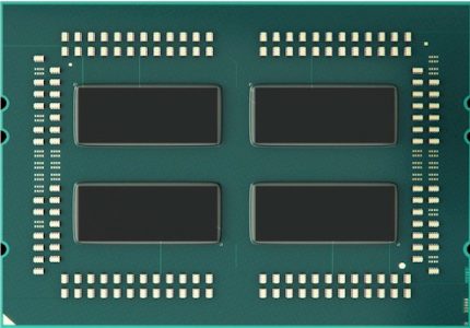
Rome is using the new 7nm Zen 2 microarchitecture. A smaller lithography process (7nm vs. 14nm) allows CPU manufacturers to cram more CPU cores in a CPU package. However, there are more elements on a CPU chip than CPU cores alone, such as I/O and memory controllers. The scalability of I/O interfaces is limited, and therefore, AMD decided to use a separated and more massive 14nm die that contains the memory and I/O controllers. This die is typically revered to as the server I/O Die (sIOD). In the picture below, you see a side by side comparison of an unlidded Naples (left) and an unlidded Rome, exposing the core chiplet dies and the SIOD. 

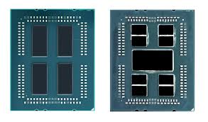
Naples Zeppelin vs. Rome Chiplet

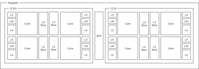
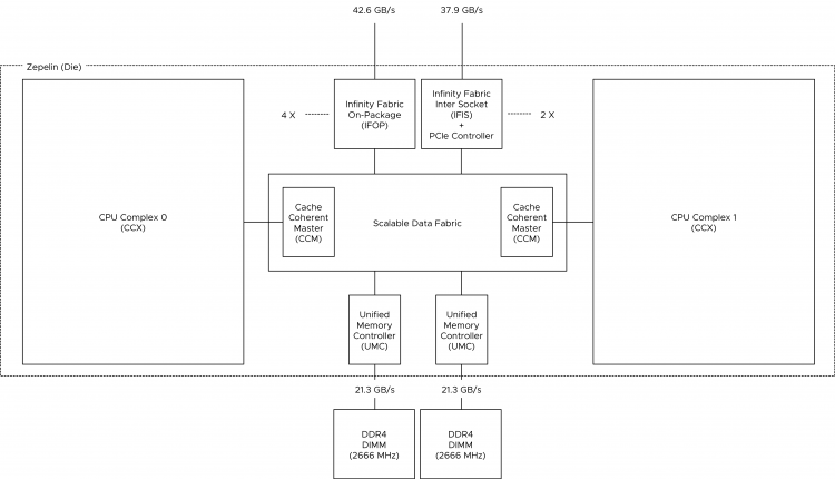
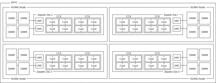
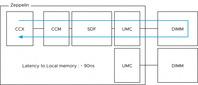
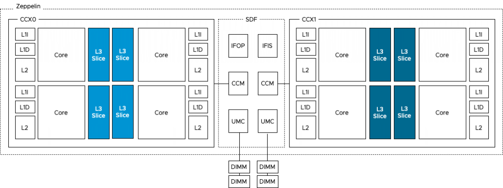
The photo above provides a clear overview of the structure of the CPU package. The Naples CPU package contains four Zeppelin dies (black rectangles). A Zeppelin die provides a maximum of eight Zen cores. The cores are divided across two compute complexes (CCX). A Zeppelin of a 32 core EPYC contains 4 cores per CCX. When Simultaneous Multi-Threading (SMT) is enabled, a CCX offers eight threads. Each CCX is connected to the Scalable Data Fabric (SDF) through the Cache-Coherent Master (CCM) that is responsible for sending traffic cross CCXes. The SDF contains two Unified Memory Controllers (UMC) connecting the DRAM memory modules. Each UMC provides a memory channel to two DIMMs. Providing the memory capacity of 4 DIMMs in total. Due to the combination of Cores, cache, and memory controller, a Zeppelin is a NUMA domain. To access a “remote” on-package memory controller, the Infinity Fabric On Package Controller (IFOP) sets up and coordinates the data communication.

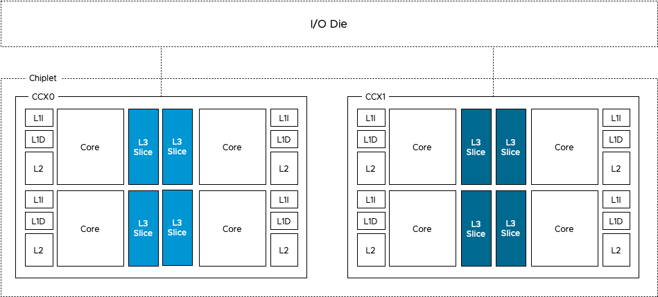
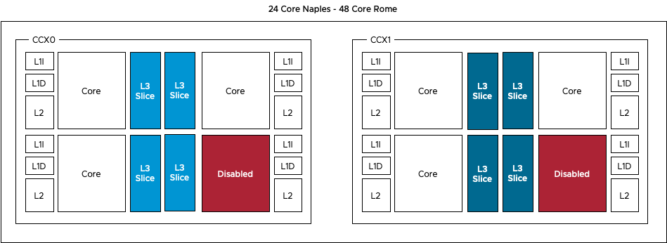
The Rome CPU package contains a 14nm I/O Die (the center black rectangle), and 8 chiplet dies (the smaller black rectangles). A Rome chiplet contains two CCX’es with each containing four cores and L3 cache, but no I/O components or the memory controllers. There is a small Infinity Fabric “controller” on each CCX that connects the CCX to the sIOD. As a result, every memory read beyond the local CCX L3 cache has to go to the sIOD. Even for a cache line (data from memory stored in the cache) that is stored in the LL3 cache of the CCX sharing the same Rome chiplet. A Chiplet is a part of the NUMA Domain.

NUMA Domain per Socket

As mentioned before, a NUMA Domain, typically called NUMA node, is a combination of CPU cores, cache, and memory capacity connected to a local memory controller. Intel architecture design uses a single NUMA Domain per Socket (NPS), AMD Naples offered four NPS, while Rome is back to a single NPS. Single NPS simplifies VM and application sizing while providing the best and consistent performance.

The bandwidth to local memory differs between each CPU architecture. The Intel Xeon Scalable Family provides a maximum of six channels of memory supporting a DDR4-2933 memory type. The Naples provides two memory channels to its locally connected memory, supporting a DDR4-2666 memory type. The Rome architecture provides eight memory channels to its locally connected memory, supporting a DDR4-3200 memory type. Please note that the memory controllers in the Rome architecture are located on the centralized die, handling all types of I/O and memory traffic, the Intel memory controllers are constructs isolated from any other traffic. Real-life application testing must be used to determine whether this architecture impacts memory bandwidth performance.

CPU Architecture	Local Channels	Mem Types	Peak transfer
Intel Xeon Scalable	6	DDR4-2666	127.8 GB/s
AMD EPYC v1 (Naples)	2	DDR4-2933	46.92 GB/s
AMD EPYC v2 (Rome)	8	DDR4-3200	204.8 GB/s

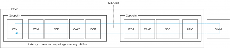
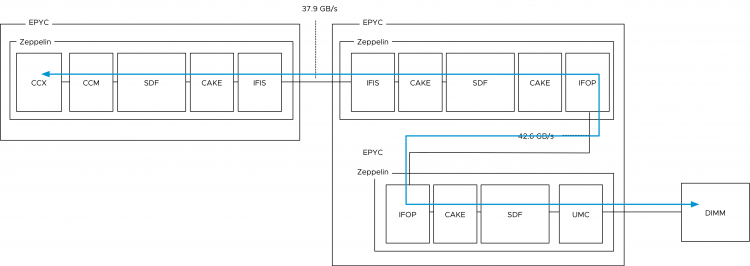
With a dual-socket system, there are typically two different distances with regards to memory access. Accessing memory connected to the local memory controller and accessing memory connected to the memory controller located on the other socket. With Naples, there are three different distances. The IFOP is used for intra-socket communication, while the Infinity Fabric Inter Socket (IFIS) controller takes care of routing traffic across sockets. As there are eight Zeppelins in a dual-socket system, not every Zeppelin is connected directly to each other and thus sometimes the memory access is routed through the IFIS first before hitting an IFOP to get to the appropriate Zeppelin. 

Naples Memory Access	Hops
Local memory access within a Zeppelin	0
Intra-socket memory access between Zeppelins	1
Inter-socket memory access between Zeppelins with direct IFIS connection	1
Inter-socket memory access between Zeppelins with indirect connection (IFIS+Remote IFOP)	2

AMD Rome provides equidistant memory access within the die and a single hop connection between sockets. Every memory access within the socket, every cache line load within the socket has to go to the I/O die. Every remote memory and cache access goes across the Infinity Fabric between sockets. This is somewhat similar to the Intel architecture that we have been familiar with since Nehalem, which launched in 2008. Why somewhat? Because there is a difference in cache domain design.

The Importance of Cache in CPU Scheduling

Getting memory capacity as close to the CPU improves performance tremendously. That’s the reason why each CPU package contains multiple levels of cache. Each core has a small but extremely fast cache capacity for instructions and data (L1), a slightly larger but relatively slower (L2) cache. A third and larger cache (L3) capacity is shared amongst the cores in the socket (Intel paradigm). Every time when a core request data to be loaded, it makes sense to retrieve this from the closest source possible, typically this is cache. To get an idea of how fast cache is relative to local and remote memory, look at the following table:

System Event	Actual Latency	Human Scaled Latency
One CPU cycle (2.3 GHz)	0.4 ns	1 second
Level 1 cache access	1.6 ns	4 seconds
Level 2 cache access	4.8 ns	12 seconds
Level 3 cache access	15.2 ns	38 seconds
Remote level 3 cache access	63 ns	157 seconds
Local memory access	75 ns	188 seconds (3min)
Remote memory access	130 ns	325 seconds (5min)
Optane PMEM Access	350 ns	875 seconds (15min)
Optane SSD I/O	10 us	7 hours
NVMe SSD I/O	25 us	17 hours

Back in the day when you could disable the cache of the CPU, someone tested the effect of cache on loading Windows 95. With cache it took almost five minutes, without the use of the cache, it took over an hour. Cache performance is crucial to get the best performance. And because of this, the vSphere NUMA scheduler and the CPU scheduler work together to optimize workloads that communicate with each other often. As they are communicating, they typically use the same data sources. Therefore, if vSphere can run the workload on the same cores that share the cache, then this could improve performance tremendously. The challenge is that AMD uses a different cache domain design than Intel.

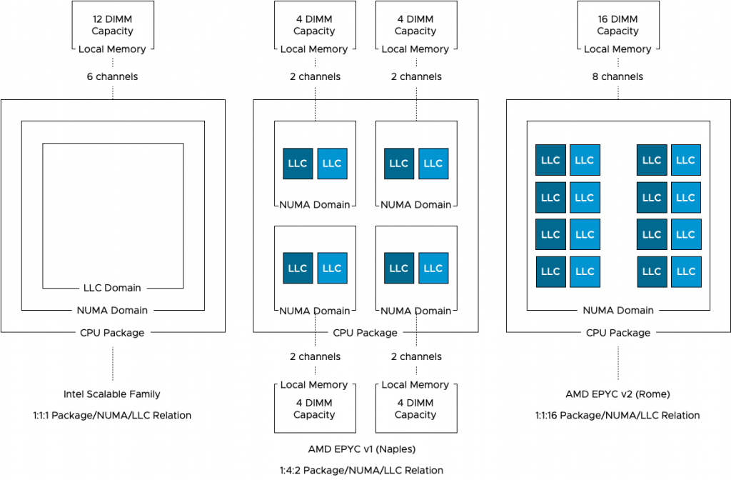
As depicted in the diagram above, Intel uses a 1:1:1 relationship model. One socket equals one NUMA domain and contains one Last Level Cache domain. As Intel is used in more than 98% of the dual-socket systems (info based on internal telemetry reports), our scheduling team obviously focused most of their efforts on this model. EPYC Naples introduced a 1:4:2 model, one socket, that contains four NUMA domains, and each NUMA domain contains two LLC domains. Rome provides a NUMA model similar to the XEON, with a single socket and single NUMA domain. However, each chiplet contains two separate LLC domains. A Rome CPU package contains eight chiplets, and thus, 16 different LLC domains exist within a socket & NUMA domain.

Relational Scheduling

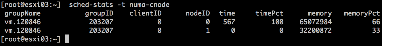
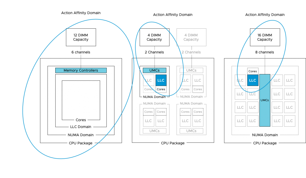
vSphere uses this LLC domain as a target for its relational scheduling functionality. Relational scheduling is better known as Action-Affinity. Its actions have made most customers think that the NUMA scheduler was broken. As the scheduler is optimized for cache sharing, it can happen that a majority of vCPU is running on a single socket, while the cores of the other sockets are idling. When reviewing ESXTOP you might see an unbalanced number of VMs running on the same NUMA Host Node (NHN). As a result, the VMs running in this NUMA domain (or in ESX terminology NHN) might compete with CPU resources and thus experience increased %Ready time.

Side note: It is my opinion to test the difference of relational scheduling on the performance of the application. Do not test this with synthetic test software. Although %Ready time is something to avoid, some applications benefit more from low-latency and highly consistent memory access than being impacted by an increase of CPU scheduling latency.

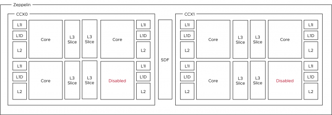
Action-Affinity can lead to ready time on an Intel CPU architecture where more than eight cores share the same cache domain, imagine what impact it can have on AMD EPYC systems where the maximum number of cores per cache domain is four. In lower-core count AMD EPYC systems, the cores are disabled per CCX, reducing the scheduling domain any further.

As the majority of the data centers are running on Intel, vSphere is optimized for a CPU topology where the NUMA and LLC domain are of consistent scope, i.e. the same size. With AMD the scopes are different and thus the current CPU scheduler can make “sub-optimal” decisions, impact performance. What happens is that the NUMA scheduler dictates the client size, the number of vCPUs to run on a NUMA Home Node, but it’s up to the CPU scheduler discretion to decide which vCPU to run on which physical core. As there are multiple Cache domains within a NUMA client, it can happen that there is an extraordinary amount of vCPU migrations between the cache domains within the NUMA domain. And that means cold cache access and a very crowded group of cores.

Therefore, the CPU team worked very hard to introduce optimizations for the AMD architecture and these optimizations are released in the updates ESXi 6.5 Update 3 and ESXi 6.7 Update 2.

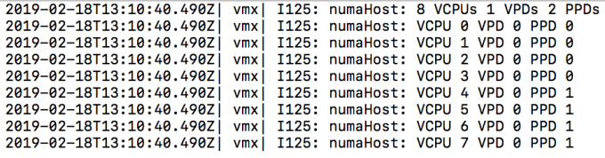
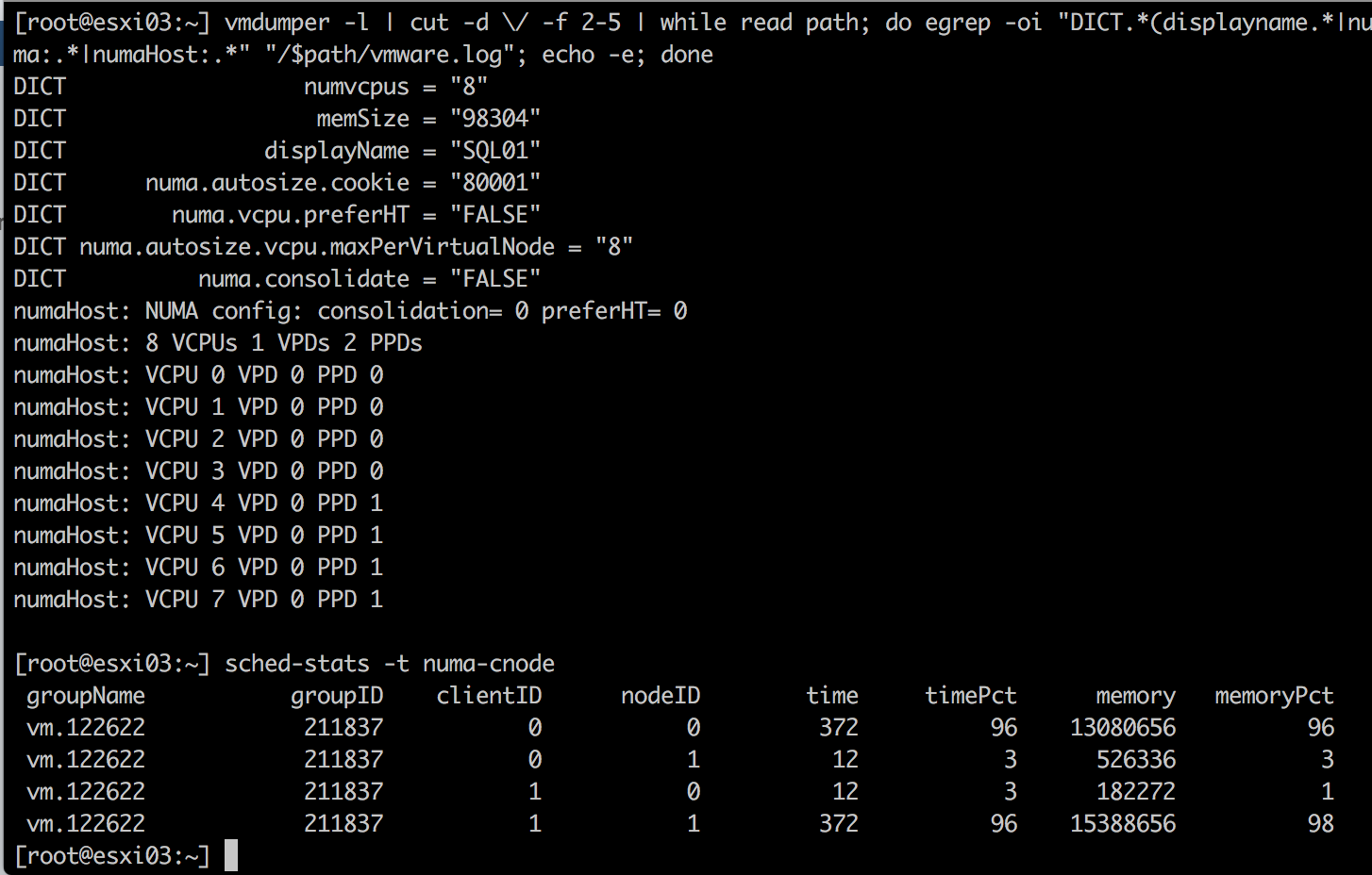
The fix informs the CPU scheduler about the presence of the multiple cache domains within the NUMA node, allowing it to schedule the vCPU more intelligently. The fix also introduces a automatic virtual NUMA client sizer. By default, a virtual NUMA architecture is exposed to the guest OS when the vCPU count exceeds the physical core count of the physical NUMA domain and if the vCPU count is no less than the numa.vcpu.min setting, which defaults to 9. A physical NUMA domain in Naples counts eight cores, and thus no virtual NUMA topology is exposed. With the patch, this is solved. What is crucial to note is that the virtual NUMA topology is determined at first boot by default. Therefore, existing VMs need to have its virtual NUMA topology reset to leverage this new functionality. This involves a power-down to remove the NUMA settings in the VMX.

When introducing Naples/Rome based systems in your virtual data center, it’s strongly recommended to deploy the latest update of your preferred vSphere platform version. This allows you to extract as much performance from your recent investment.

AMD is gaining popularity in the server market with the EPYC CPU platform. The EPYC CPU platform provides a high core count and a large memory capacity. If you are familiar with previous AMD generations, you know AMD’s method of operation is different than Intel’s. For reference, take a look at the article I wrote in 2011 about the 12-core 6100 Opteron code name Magny-Cours. EPYC provides an increase of scale but builds on the previously introduced principles. Let’s review the EPYC architecture and see how it can impact your VM sizing and ESXi configuration. (Please note that this article is NOT intended as a good/bad comparison between AMD and Intel, I’m just describing the architectural differences).

EPYC Architecture
The EPYC processor architecture is what AMD refers to as a Multi-Chip-Module (MCM). EPYC is designed to provide a high core count platform by combining multiple silicon dies within a CPU Package. A silicon die (named Zeppelin) is a wafer that contains the circuitry. In simple terms, it’s the component that contains CPU cores, memory cache, and various controllers. Regardless of the core-count, an EPYC CPU package always contains four Zeppelin dies. Comparing this to Intel Xeon, a Xeon CPU package is a single-chip-design which consist of a single silicon die containing all components. The reason why the difference in chip design is interesting is that impacts the logical grouping of compute resources. The size of the logical group, better known as a NUMA node, impacts scheduling decisions made by the CPU scheduler of the operating system (both the hypervisor kernel and possibly the guest operating system). It might be necessary to change some of the default settings of the ESXi host to alter scheduling behavior, these settings are covered in the last part of the article. Let’s continue to explore the architecture of the EPYC CPU.

Compute Complex
The photo above provides a clear overview of the structure of the CPU package. The CPU package houses four Zeppelin dies. In the current generation, a Zeppelin die provides a maximum of eight Zen cores. The cores are divided across two compute complexes (CCX). A Zeppelin of a 32 core EPYC contains 4 cores per CCX. When Simultaneous Multi-Threading (SMT) is enabled within the BIOS, a CCX offers eight threads.

Each core has its own L1 (instruction (64KB) and data (32KB)) and L2 caches (4 MB total L2 cache). A Zeppelin has 16 MB L3 cache. Interestingly enough, each CCX has it’s own L3 Cache of 8MB, in turn, split up into four slices of 2 MB. The two CCXes within a Zeppelin die are connected to each other through an interconnect (Infinity Fabric). Adding hops to memory access is not beneficial to bandwidth and latency. Multiple tech-sites have performed in-depth testing on cache performance, and to quote Anandtech.com:

“The local “inside the CCX” 8 MB L3-cache is accessed with very little latency. But once the core needs to access another L3-cache chunk – even on the same die – unloaded latency is pretty bad: it’s only slightly better than the DRAM access latency.” 

In essence, this means that you cannot think of the 64MB L3 cache as one single pool of cache capacity. Better is to approach it as eight 8MB capacity pools. This is important to realize if multiple workloads share the same data, the NUMA scheduler of ESXi attempts to place both workloads in the same NUMA node to optimize cache and memory performance for these workloads. It might happen that the L3 cache size is not sufficient enough. The option that impacts this behavior is called Action Affinity, more details about this setting can be found in the last part of the article.

Zeppelin Core Count
EPYC is offered in multiple SKUs. Next, to the 32 core count model, there are lower-core count models. Since the EPYC architecture always includes four Zeppelins, the difference in core count is created by disabling cores per CCX in a symmetrical way. For example, in a 24 core count EPYC, a single Zeppelin die would look like this.

The table shows the core count per Zeppelin of the three largest EPYC CPUs. The total cores per Zeppelin count can be used as a guideline for the vNUMA setting described later in this article

Cores	Cores per CCX	Total Cores per Zeppelin	Zeppelin Count
32	4	8	4
24	3	6	4
16	2	4	4

Infinity Fabric
The cores within a CCX communicate with memory (DIMMs) via an on-die memory controller through the infinity Fabric. The Infinity fabric is AMD’s proprietary system interconnect architecture that facilitates data and control transmission across all linked components. The Infinity Fabric consists of two communication planes; the Scalable Data Fabric (SDF) and the Infinity Scalable Control Fabric (SCF). The SCF is responsible for processing system control signals, such as thermal and power management. Although very important, we are more interested in the SDF which is responsible for transmitting data within the system. The rest of the article zooms into SDF design and its impact on scheduling decisions.

Each CCX is connected to the SDF through the Cache-Coherent Master (CCM) that is responsible for sending coherent data traffic cross CCXes. The SDF uses a Unified Memory Controller (UMC) to connect to DRAM memory modules. Each UMC provides a memory channel to two DIMMs. Providing the memory capacity of 4 DIMMs in total.

How does this design impact VM sizing? A Zeppelin is a NUMA node that contains a maximum of 8 cores (16 threads) with the memory capacity of four DIMMs. This design results in a single EPYC CPU package presents four NUMA nodes to the operating system.

Server Memory Capacity and NUMA
Intel moved from a 3 DIMMs per channel configuration (DPC) with 4 channels to a model with 6 channels and 2 DIMMs deep. This new model broke the capacity model cadence. For example, using 16 GB DIMMs, you had either 64 GB, 128GB or 192GB available per socket. Now with the scalable architecture, it’s either 96GB or 192GB. That is if you follow the high- performance best practice of populating all channels for maximum bandwidth availability. However, with the current DIMM pricing, a lot of customers cannot afford such a configuration.

With the EPYC, every Zeppelin has two memory channels. Each memory channel can drive two DIMMs. For good performance, each Zeppelin should be equipped with at least 1 DPC. That means that a proper performing dual socket EPYC system should be configured with 16 DIMMs. This configuration allows for a theoretical bandwidth of 42.6 GB/s while providing a (shallow) memory capacity of just the two DIMMs combined. This design results in a single EPYC CPU package presents four NUMA nodes to the operating system. If the minimum of 1DPC is used, the NUMA node size can be too small and thus the overall performance if the VM memory size exceeds the physical memory configuration of each Zeppelin. Servethehome published some benchmark tests about the performance difference between the different memory configurations of EPYC.

With NUMA, it’s important to understand the boundaries of your local memory domain and your remote memory domain. Traditionally the domains were easily demarcated by the CPU package core count and attached memory capacity. With EPYC, a new distinction has to be made between the different remote memory access types. It can be remote on-package memory access or remote socket memory access. The reason why this distinction has to be made is the impact on performance and consistency of application memory access. Having your VM and application span multiple NUMA nodes can introduce a very inconsistent response time.

Local Memory Access 
Let’s start with the best and most consistent performance. When a core within the Zeppelin access local memory the path is as follows:

The presentation “Zeppelin an SOC for Multi-Chip Architectures” by AMD list the latency of local memory access within the Zeppelin at 90 nanoseconds.

Remote Memory Access On Package
A core can access memory attached to a different Zeppelin within the same CPU package. This is called remote on-package memory access or “on-package Die-to-Die” memory access. This means we are still using memory controllers within the same socket. In total the EPYC CPU has eight memory channels, but two are local to the Zeppelin. To access a “remote” on-package memory controller the Infinity Fabric On Package Controller (IFOP) sets up and coordinates the data communication.

In total each Zeppelin has 4 IFOPs, but actually, only three are needed since there are 3 other Zeppelins within the same CPU package.

To be more precise, the IO traverses an additional component before hitting the IFOP. This component is called the Coherent AMD socKet Extender (CAKE). It facilitates die-to-die or socket-to-socket memory transactions. This module translates the request and response formats used by the SDF transport layer to and from the serialized format used by the IFOP. What that means is that a few extra hops and CPU cycles are introduced when fetching data stored within DIMMs attached to other Zeppelins on the same die. AMD reports a latency of ~145ns.

Inter Package Remote Access
And then we have the chance that memory needs to be fetched from DIMMs attached to UMCs from a Zeppelin that is a part of another EPYC CPU package within the system (dual socket system). Instead of routing the traffic across the IFOP, the traffic is routed across Infinity Fabric Inter Socket (IFIS) controller. Package-to-package traffic has 8/9 of the bandwidth of IFOP traffic, resulting in a theoretical bandwidth of 37.9 GB/s. The reduction in bandwidth increases the chance of experiencing inconsistent performance. The increased length of the path, increments latency. AMD reports a latency of ~200ns.

Because there are two IFIS controllers per Zeppelin, not every Zeppelin within a dual socket system is directly connected to each other. In the worst case scenario, there are two hops. One hop from one package to the other package and an extra hop to go from one Zeppelin to the Zeppelin that is connected to the DIMM holding the data. Unfortunately, AMD as not shared latency data.

VM Sizing
The key is to keep memory access as much local as possible. ESXi and most modern guest operating systems are optimized to deal with NUMA. However as with most things in life, for the most optimal performance, reduce distance and reduce any form of variation. Apply this to VM sizing and try to keep the vCPU count of a VM within the core count of NUMA domain. Same applies to VM memory capacity, try to fit this with the capacity of the NUMA node. If the VM cannot fit inside a NUMA node, there is no need to stress, ESXi has got the best NUMA scheduler in the business. To help ESXi to optimize for the EPYC architecture, some advanced settings might be necessary to adjust. As always, tests these settings in a non-revenue critical environment before applying them to production systems.

Virtual NUMA
Virtual NUMA (vNUMA) allows the operating system to understand the “physical” layout of the virtual machine. vNUMA presents the mapping of the VM vCPU to the physical NUMA nodes of the ESXi host. For example, if a VM has 12 vCPUs and the physical core count within a single NUMA node was 10 cores, ESXi would present the guest OS a topology of 2 NUMA nodes with each counting 6 cores. ESXi would group 6 vCPUs into a NUMA client and schedule these across the 10 CPU cores within a NUMA node.

When vNUMA was introduced, the highest core count of a CPU was 8 CPUs, thus the VMware engineers introduced a vNUMA threshold of 9 (numa.vcpu.min=9). Meaning that the VM needs to contain at least 9 vCPUs in order to generate the virtual NUMA topology.Considering the highest core-count of an EPYC system is eight cores per Zeppelin, you might want to adjust the vNUMA default threshold to resemble the physical layout of the used EPYC model.

For example, the EPYC 7401 contains 24 cores, 6 cores per Zeppelin and thus 6 cores per NUMA node. When using the default setting of numa.vcpu.min=9, an 8 vCPU VM is automatically configured like this.

A VPD is the virtual NUMA client that is exposed to the guest OS system, while a PPD is the NUMA client used by the VMkernel CPU scheduler. In this situation, the ESXi scheduler uses two physical NUMA nodes to satisfy CPU and memory requests while the guest OS perceives the layout as a Uniform Memory Access (UMA) system. In a UMA system, the access time to a memory location is independent of which processor makes the request, or which memory chip contains the transferred data). I.e., pretty much the same latency and bandwidth throughout the system. However, this is not the case as reported in this article above. Reading and writing remote CCX cache and remote memory (on-die) is slower than local memory even within the same Zeppelin. By setting the numa.vcpu.min=6, two VPDs are created, and thus the guest OS is made aware of the physical layout by the ESXi scheduler. The guest OS and the applications can optimize memory operations to attain consistent performance.

Action Affinity
When the ESXi scheduler detects multiple VMs communicating with each other, it can decide of placing them together on the same NUMA node to increase intra-NUMA node communication. This behavior is called action affinity, and it can increase performance by up to 30%. However, with the small NUMA nodes of max 8 CPUs, it can also lead to a lot of cache thrashing and remote memory access if the configured memory of the VMs cannot fit inside a single NUMA node. If this is the case, it might be helpful to test disabling the action affinity on the ESXi host. This is done by configuring the /Numa/LocalityWeightActionAffinity to 0 (KB 2097369).

What if the VM Memory Config Exceeds the Memory Capacity of the Physical NUMA Node?
I wrote an article about this situation back in 2017, and it’s featured in the vSphere 6.5 Host deep dive book. However, what happens if your VM memory configuration exceeds the physical capacity of a NUMA node. By default, the ESXi scheduler optimizes for local memory access and attempts to place as much memory along with the vCPU in the same NUMA node. Sometimes it can improve local memory access to creating multiple smaller NUMA clients.

For example, on an EPYC 7601 (32 core), the NUMA node contains 8 cores, and this server is equipped with 256 GB by using 16 x 16 GB DIMMs. A NUMA node has 4 DIMMs attached to it. Thus the NUMA node provides 8 cores and 64 GB. What happens if a VM is configured with 6 vCPUs and 96 GB? By default the NUMA scheduler attempts to store 64GB of VM memory inside the NUMA node, leaving 32 GB in a remote NUMA node. By enabling the VM advanced setting numa.consolidate = FALSE. It instructs the NUMA scheduler to distribute the VM configuration across the optimal number of NUMA nodes greater than 1. In this case, 2 NUMA clients are created, and this will schedule 3 vCPUs in each NUMA node.

Now the performance and the behavior of the application depends on its design. If you have a single-threaded application, this setting might not be helpful at all. However, if it’s a multi-threaded application, you might see some benefit. The only thing to do is to set the numa.vcpu.min equal to the number of vCPUs per virtual NUMA client to expose the vNUMA architecture to the guest OS and the application. The following command helps you to retrieve the NUMA configuration of the VM:

vmdumper -l | cut -d \/ -f 2-5 | while read path; do egrep -oi “DICT.(displayname.|numa.|cores.|vcpu.|memsize.|affinity.)= .|numa:.|numaHost:.” “/$path/vmware.log”; echo -e; done

Please bear in mind that the ESXi CPU and NUMA scheduler do not use an SRAT (System Resource Allocation Table) to determine the distance of the individual NUMA nodes between each other. ESXi uses its own method to determine latency between the different NUMA nodes within the system. It uses these latency numbers for initial placement and attempts to schedule the NUMA clients of a VM as close to each other as possible. However, the ESXi scheduler does not leverage this information during load-balancing operations. This is work in progress. Adding a new first class metric to a heuristic is not a simple task and knowing the CPU engineers, they want to provide a system that is thoroughly improved by augmenting new code.

Increase NUMA Node Compute Sizing
For workloads that are memory latency sensitive with a low processor utilization, you can alter the way the NUMA scheduler sizes the NUMA client of that particular VM. The VM advanced setting numa.vcpu.preferHT=TRUE allows the NUMA scheduler to count threads instead of cores for NUMA node size configuration. For example, an 8 vCPU VM that uses this advanced setting and runs on an EPYC 7401 system (6 cores, 12 threads), is scheduled within a single Zeppelin.
If all workloads follow the same utilization pattern, you can alter the ESXi host setting by adding numa.PreferHT=1 to the ESXi host advanced configuration.

Channel-Pair Interleaving (1 NUMA node per socket)
The EPYC architecture can interleave the memory channels and thus present the cores of the four zeppelins as a single NUMA node. This setting requires that every channel is populated with equal memory size. Some vendors use a different name for it. For example, Dell calls this setting “Memory Die Interleaving”. Little to no data can be found about the performance impact of this setting, but keep in mind, software settings do not change the physical layout (and thus physics). Typically abstraction filters out the outliers and presents an average performance behavior. For NUMA benchmarking, please take a look at the article “AMD EPYC – STREAM, HPL, InfiniBand, and WRF Performance Study” located on the Dell website.

Research Your Workload Requirements
ESXi can handle complex NUMA architectures as the best. However, it’s always best to avoid complexity as possible. Determine if your workload can fit in a minimum number of small NUMA nodes when using the EPYC architecture? Can the workload handle inconsistent memory performance if it does exceed the NUMA node size of 8? The EPYC architecture is an excellent way of adding scale to the server platform but do remember that for real-life workload optimal performance is achieved when you take the NUMA configuration boundaries into account.

On Twitter some asked what my thoughts are about the EPYC CPU architecture? For every tech challenge, there is a solution. When looking at the architecture, I think EPYC is an excellent solution for small and medium-sized workloads. I expect that larger monolithic apps, that require consistent performance, are better off looking at different architectures. (My opinion, not VMware’s!)

This week I had the pleasure to talk to a customer about NUMA use-cases and a very interesting config came up. They have a VM with a particular memory configuration that exceeds the ESXi host NUMA node memory configuration. This scenario is covered in the vSphere 6.5 Host Resources Deep Dive, excerpt below.

Memory Configuration
The scenario described happens in multi-socket systems that are used to host monster-VMs. Extreme memory footprint VMs are getting more common by the day. The system is equipped with two CPU packages. Each CPU package contains twelve cores. The system has a memory configuration of 128 GB in total. The NUMA nodes are symmetrically configured and contain 64 GB of memory each.

However, if the VM requires 96 GB of memory, a maximum of 64 GB can be obtained from a single NUMA node. This means that 32 GB of memory could become remote if the vCPUs of that VM can fit inside one NUMA node. In this case, the VM is configured with 8 vCPUs.

The VM fits from a vCPU perspective inside one NUMA node, and therefore the NUMA scheduler configures for this VM a single virtual proximity domain (VPD) and a single a load-balancing group which is internally referred to as a physical proximity domain (PPD).

Example Workload
Running a SQL DB on this machine resulted in the following local and remote memory consumption. The VM consumes nearly 64 GB on its local NUMA node (clientID shows the location of the vCPUs) while it consumes 31 GB of remote memory.

In this scenario, it could be beneficial to the performance of the VM to rely on the NUMA optimizations that exist in the guest OS and application. The VM advanced setting numa.consolidate = FALSE instructs the NUMA scheduler to distribute the VM configuration across as many NUMA nodes as possible.

In this scenario, the NUMA scheduler creates 2 load-balancing domains (PPDs) and allows for a more symmetrical configuration of 4 vCPUs per node.

Please note that a single VPD (VPD0) is created and as a result, the guest OS and the application only detect a single NUMA node. Local and remote memory optimizations are (only) applied by the NUMA scheduler in the hypervisor.

Whether or not the application can benefit from this configuration depends on its design. If it’s a multi-threaded application, the NUMA scheduler can allocate memory closes to the CPU operation. However, if the VM is running a single-threaded application, you still might end up with a lot of remote memory access, as the physical NUMA node hosting the vCPU is unable to provide the memory demand by itself.

Test the behavior of your application before making the change to create a baseline. As always, use advanced settings only if necessary!

The Intel Xeon Scalable Family introduces a new platform (Purley). The most prominent change regarding system design is the memory subsystem.
More Memory Bandwidth and Consistency in Speed
The new memory subsystem supports the same number of DIMMs per CPU as the previous models. However, it’s wider and less deep. What I mean by that is that the last platform (Grantley) supported up to three DIMMs per channel (DPC) and made use of four channels. In total, the Grantley platform supported up to twelve DIMMs per CPU. Purley increases the number of channels from four to six but reduces the numbers of supported DIMMs per channel from three to two. Although this sounds like a potato, potato; tomato, tomato discussion it provides a significant increase in bandwidth while ensuring consistency in speed during a scaling up exercise. Let’s take a closer look.
DIMMs per Memory Channel
Depending on the DIMM slot configuration of the server board, multiple DIMMs are supported per channel. The E5-2600 V-series supports up to 3 DIMMs per channel (3 DPC). Using more DIMMs per channel provides the largest capacity, but unfortunately, it impacts the operational speed of memory.

A DIMM groups memory chips into ranks. DIMMs come in three rank configurations; single-rank, dual-rank or quad-rank configuration, ranks are denoted as (xR). With the addition of each rank, the electrical load on the channel increases. And as more ranks are used in a memory channel, memory speed drops restricting the use of additional memory. Therefore in certain configurations, DIMMs will run slower than their listed maximum speeds. This reduction in speed occurs when 3 DIMMs per channel is used.

RDIMM	1 DPC	2 DPC	3 DPC	LRDIMM	1 DPC	2 DPC	3 DPC	Source
Cisco	2400 MHz	2400 MHz	1866 MHz		2400 MHz	2400 MHz	2133 MHz	Cisco PDF
Dell	2400 MHz	2400 MHz	1866 MHz		2400 MHz	2400 MHz	2133 MHz	Dell.com
Fujitsu	2400 MHz	2400 MHz	1866 MHz		2400 MHz	2400 MHz	1866 MHz	Fujitsu PDF
HP	2400 MHz	2400 MHz	1866 MHz		2400 MHz	2400 MHz	2400 MHz*	HP PDF
Performance Drop	0	0	28%		0	0	12%/28%

* HP claims no reduction of speed due to proprietary memory technology. I have not tested this.
Moving to 2 DIMMs per Channel Configuration
The Purley platform avoids this pitfall by reducing the supported number of DIMMs per channel. It supports up to 2 DIMMs per channel, maintaining the same performance regardless the number of DIMMs per channel. However, reducing the number of DIMMs supported per channel severely impacts the total supported memory capacity per CPU. Intel solves this by adding more channels to the memory controller. For some organizations, this change can result in dropping the requirement of obtaining LRDIMMs. Some organizations avoid the steep performance reduction by purchasing the (more) expensive LRDIMMs, 2 DPC configurations will not affect the performance characteristics of the memory modules.
Six Memory Channel Support
The Purley platform supports up to six channels per CPU. As a result, the bandwidth increases and the support for high capacity memory systems remains. By default, the new Xeon CPU supports up to 768 GB. Please review part 1 of this series in which covers the high memory capacity optimization option (M-suffix).

If all six channels are populated with DIMMs, the CPU interleaves memory access across the multiple memory channels. When creating a 1 DIMM per channel (1 DPC) configuration, the CPU forms one region (Region 0) and interleaves the memory access. Theoretically, this multiplies the data rate by exactly the number of channels present. A 2666 MT/s DIMM has a theoretical peak transfer rate of 21,300 MB/s. If populating all six DIMM slots, the memory controller accesses each module sequentially. Instead of writing all the data to a single DIMM, the data is written across the modules in one region in an alternating pattern, leveraging each channel bandwidth separately. That means that the memory controllers of a single Xeon CPU have access to a combined bandwidth of 127,800 MB/s. In theory, that means that a dual Xeon system has access to 256 GB per second (21,300 MB/s x 6 channels x 2 sockets). In theory!
This all depends on the type of workload and the compute power that drives the workload. The Xeon’s cores have direct access to the six channels in the CPU package. One thread can never obtain 256 GB due to the interconnect and the raw power it can produce to feed the channels. Anandtech has an excellent write-up about this behavior.
Memory Configuration
As a result of an increase of channels and the design consideration of populating every DIMM slot to create a 1 DPC or 2 DPC configuration, a new vSphere system will likely have a different memory capacity configuration than your previous systems (Inform your standards commission). Please note that the table lists the memory configuration of a single NUMA node.

6 x DIMM	16 GB	32 GB	64 GB	128 GB
1 DPC	96 GB	192 GB	384 GB	768 GB
2 DPC	192 GB	384 GB	768 GB	1536 GB *

* M-suffix Xeon CPU required
Please note that the table lists the memory configuration of a single NUMA node. Dual CPU systems is the most common configuration for vSphere servers. That means that you can expect the major system integrators such as DELL and HP to offer the following configurations:

Dual CPU Socket	16 GB	32 GB	64 GB	128 GB
1 DPC	192 GB	384 GB	768 GB	1536 GB
2 DPC	384 GB	768 GB	1536 GB	3072 GB *

For completeness sake, the next table shows the configuration of a v4 system with a maximum of 2-DPC. Very familiar configuration numbers, I guess we just need to get used to the new configuration standards such as 384, 768 and 1536 GB per system.

Dual CPU Socket v4	16 GB	32 GB	64 GB	128 GB
1 DPC	128 GB	256 GB	512 GB	1024 GB
2 DPC	256 GB	512 GB	1024 GB	2048 GB

* M-suffix Xeon CPU required.
vSphere 6.5 supports up to 12 TB per host. As a result, the entire range of Intel Xeon Scalable CPU with the extended memory feature is fully supported (8 CPUs x 1536 GB). Interesting data point, the vSphere 6.5 Configurations Maximum Guide started to list a maximum number of NUMA nodes per system. This limit is set to 16. The Intel Scalable Xeon supports sub-NUMA clustering (similar to Cluster-on-Die functionality), splitting up the CPU package into two NUMA nodes. As a result, vSphere 6.5 would support a system equipped with 8 Intel Xeon Platinum 8176M Processors each fully loaded with 1.5 TB of memory and configured with sub-NUMA clustering. This setup would create one system, offering 16 NUMA nodes each fitted with 768 GB of local memory.
Take Caution of 8 DIMM System Board Designs
The introduction of Purley forces system integrators to redesign the system boards to support the new functionality. To support the full possibilities of the memory subsystem, system boards should be equipped with either 6 or 12 DIMM sockets. Some entry-level systems are designed with 8 DIMM slots. The Intel Xeon is designed to use the six channels when creating a region, this results in an unbalanced region design of 6+2. Region 0 consists of 6 DIMM slots, offering a theoretical peak transfer rate of 127,800 MB/s (when using 2666 GT/s), while region 1 offers
42,600 MB/s. This will result in inconsistent performance, something to definitely to avoid. Thus it’s recommended to equip these systems with the six-channel configuration in mind, order these systems and only populate the first six DIMM slots per CPU.
Interconnect
The performance of a dual CPU system can be impacted by the interconnect between the CPU packages if you span VMs across the NUMA nodes (Wide-VMs). Purley introduces a new interconnect called the UltraPath Interconnect (UPI) and replaces the QuickPath Interconnect. The next article in this series provides an in-depth look at the UPI.