Reviewing the physical layers helps to understand the behavior of the CPU scheduler of the VMkernel. This helps to select a physical configuration that is optimized for performance. This part covers the Intel Xeon microarchitecture and zooms in on the Uncore. Primarily focusing on Uncore frequency management and QPI design decisions.

Terminology

There a are a lot of different names used for something that is apparently the same thing. Let’s review the terminology of the Physical CPU and the NUMA architecture. The CPU package is the device you hold in your hand, it contains the CPU die and is installed in the CPU socket on the motherboard. The CPU die contains the CPU cores and the system agent. A core is an independent execution unit and can present two virtual cores to run simultaneous multithreading (SMT). Intel proprietary SMT implementation is called Hyper-Threading (HT). Both SMT threads share the components such as cache layers and access to the scalable ring on-die Interconnect for I/O operations.

Interesting entomology; The word “die” is the singular of dice. Elements such as processing units are produced on a large round silicon wafer. The wafer is cut “diced” into many pieces. Each of these pieces is called a die.

NUMA Architecture

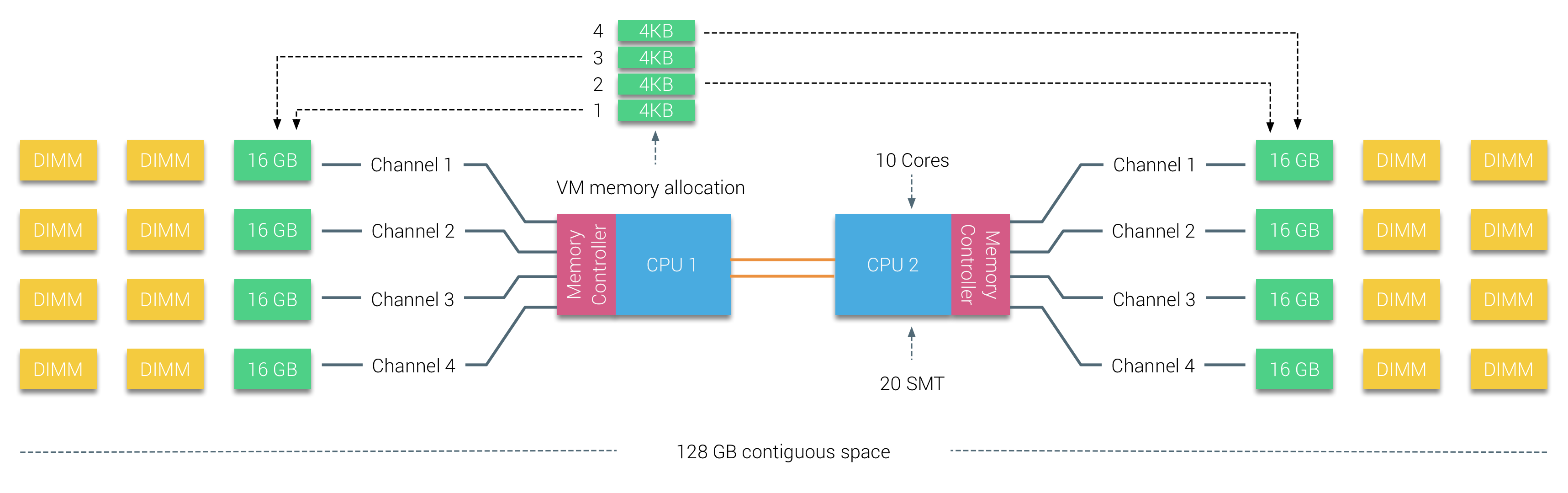
In the following scenario, the system contains two CPUs, Intel 2630 v4, each containing 10 cores (20 HT threads). The Intel 2630 v4 is based on the Broadwell microarchitecture and contains 4 memory channels, with a maximum of 3 DIMMS per channel. Each channel is filled with a single 16 GB DDR4 RAM DIMM. 64 GB memory is available per CPU with a total of 128 GB in the system. The system reports two NUMA Nodes, each NUMA nodes, sometimes called NUMA domain, contains 10 cores and 64 GB.

Consuming NUMA

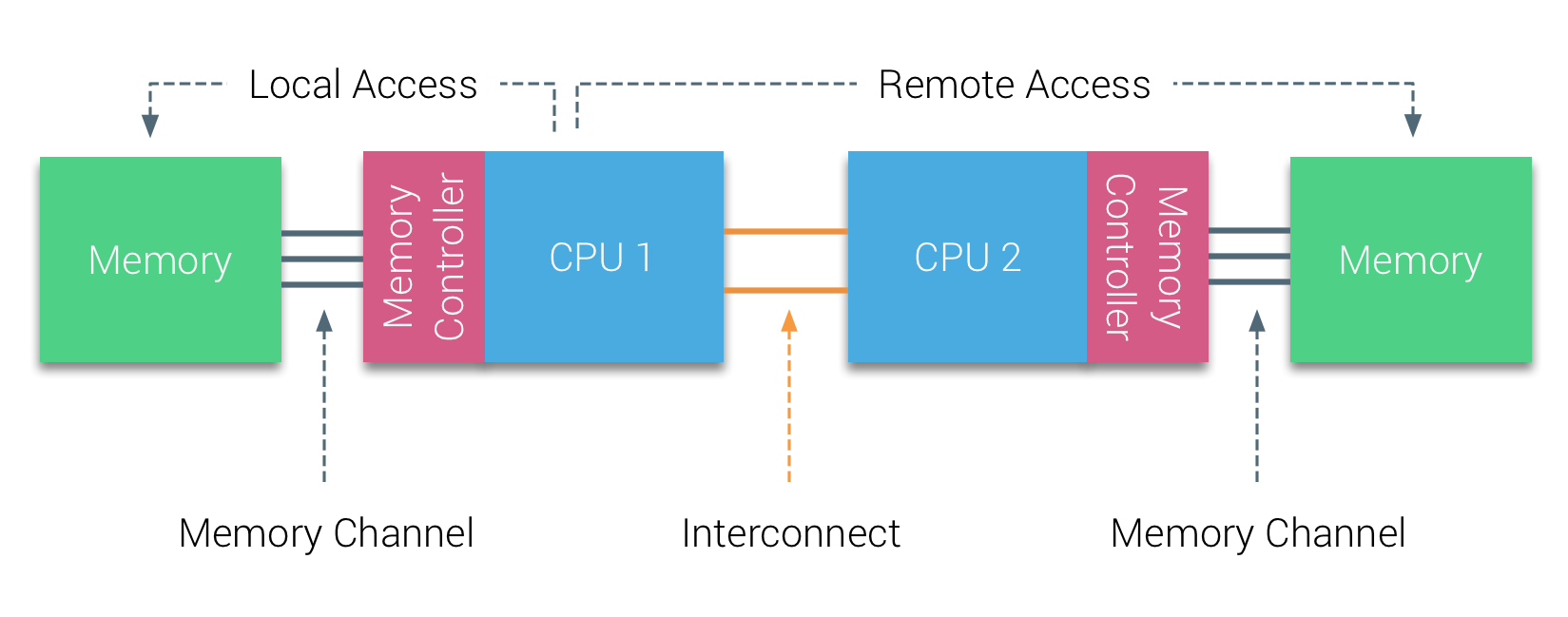
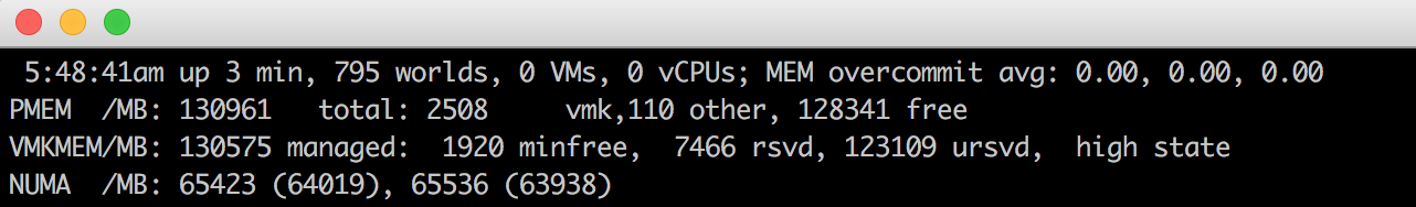
The CPU can access both its local memory and the memory controlled by the other CPUs in the system. Memory capacity managed by other CPUs are considered remote memory and is accessed through the QPI (Part 1). The allocation of memory to a virtual machine is handled by the CPU and NUMA schedulers of the ESXi kernel. The goal of the NUMA scheduler is to maximize local memory access and attempts to distribute the workload as efficient as possible. This depends on the virtual machine CPU and memory configuration and the physical core count and memory configuration. A more detailed look into the behavior of the ESXi CPU and NUMA scheduler is done in part 5, how to size and configure your virtual machines is discussed in part 6. This part focusses on the low-level configuration of a modern dual-CPU socket system. ESXtop reports 130961 MB (PMEM /MB) and displays the NUMA nodes with its local memory count.

Each core can address up to 128 GB of memory, as described earlier the NUMA scheduler of the ESXI kernel attempts to place and distribute vCPU as optimal as possible, allocating as much local memory to the CPU workload that is available. When the number of VCPUs of a virtual machine exceeds the core count of a physical CPU, the ESXi server distributes the vCPU even across the minimal number of physical CPUs.It also exposes the physical NUMA layout to the virtual machine operating system, allowing the NUMA-aware operating system and / or application to schedule their processes as optimal as possible. To ensure this all occurs, verify if the BIOS is configured correctly and that the setting NUMA = enabled or Node Interleaving is disabled. In this example a 12 vCPU VM is running on the dual Intel 2630 v4 system, each containing 10 cores. CoreInfo informs us that 6 vCPUs are running on NUMA node 0 and 6 vCPUs are running on NUMA node 1.

BIOS Setting: Node Interleaving

There seems to be a lot of confusion about this BIOS setting, I receive lots of questions on whether to enable or disable Node interleaving. I guess the term “enable” make people think it some sort of performance enhancement. Unfortunately, the opposite is true and it is strongly recommended to keep the default setting and keep Node Interleaving disabled.

Node Interleaving Disabled: NUMA
By using the default setting of Node Interleaving (disabled), the ACPI “BIOS” will build a System Resource Allocation Table (SRAT). Within this SRAT, the physical configuration and CPU memory architecture are described, i.e. which CPU and memory ranges belong to a single NUMA node. It proceeds to map the memory of each node into a single sequential block of memory address space. ESXi uses the SRAT to understand which memory bank is local to a physical CPU and attempts to allocate local memory to each vCPU of the virtual machine.

Node Interleaving Enabled: SUMA
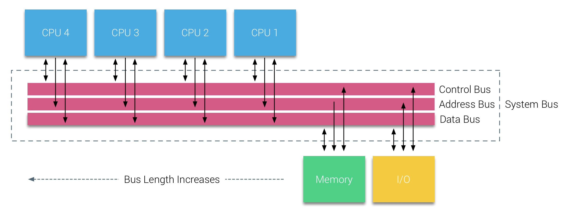
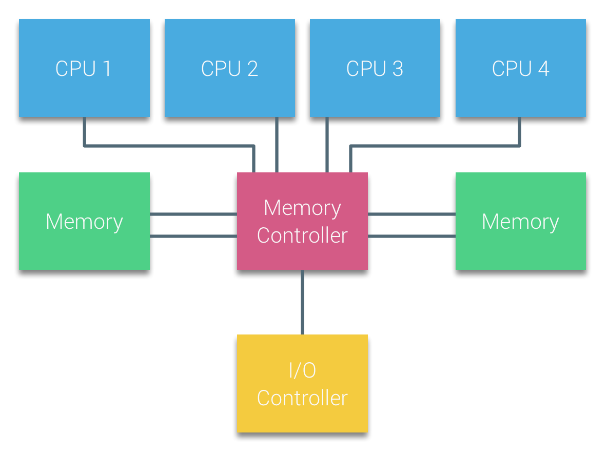
One question that is asked a lot is how do you turn off NUMA? You can turn off NUMA, but remember your system is not a transformer, changing your CPUs and memory layout from a point-to-point-connection architecture to a bus system. Therefore, when enabling Node Interleaving the system will not become a traditional UMA system. Part 1 contains a more info on SUMA.

BIOS setting: ACPI SLIT Preferences
The ACPI System Locality Information Table (SLIT) provides a matrix that describes the relative distance (i.e. memory latency) between the proximity domains. In the past, a large NUMA system the latency from Node 0 to Node 7 can be much greater than the latency from Node 0 to Node 1, and this kind of information is provided by the SLIT table.

Modern point-to-point architectures moved from a ring topology to a full mesh topology reducing hop counts, reducing the importance of SLIT. Many server vendor whitepapers describing best practices for VMware ESXi recommend enabling ACPI SLIT. Do not worry if you forgot to enable this setting as ESXi does not use the SLIT. Instead, the ESXi kernel determines the inter-node latencies by probing the nodes at boot-time and use this information for initial placement of wide virtual machines. A wide virtual machine contains more vCPUs than the Core count of a physical CPU, more about wide virtual machines and virtual NUMA can be found in the next article.

CPU System Architecture

Since Sandy Bridge (v1) the CPU system architecture applied by Intel can be described as a System-on-Chip (SoC) architecture, integrating the CPU, GPU, system IO and last level cache into a single package. The QPI and the Uncore are critical components of the memory system and its performance can be impacted by BIOS settings. Available QPI bandwidth depends on the CPU model, therefore it’s of interest to have a proper understanding of the CPU system architecture to design a high performing system.

Uncore

As mentioned in part 1, the Nehalem microarchitecture introduced a flexible architecture that could be optimized for different segments. In order to facilitate scalability, Intel separated the core processing functionality (ALU, FPU, L1 and L2 cache) from the ‘uncore’ functionality. A nice way to put it is that the Uncore is a collection of components of a CPU that do not carry out core computational functions but are essential for core performance. This architectural system change brought the Northbridge functionality closer to the processing unit, reducing latency while being able to increase the speed due to the removal of serial bus controllers. The Uncore featured the following elements:

Uncore element	Description	Responsible for:
QPI Agent	QuickPath Interconnect	QPI caching agent , manages R3QPI and QPI Link Interface
PCU	Power Controller	Core/Uncore power unit and thermal manager, governs P-state of the CPU, C-state of the Core and package. It enables Turbo Mode and can throttle cores when a thermal violation occurs
Ubox	System Config controller	Intermediary for interrupt traffic between system and core
IIO	Integrated IO	Provides the interface to PCIe Devices
R2PCI	Ring to PCI Interface	Provides interface to the ring for PCIe access
IMC	Integrated Memory Controller	Provides the interface to RAM and communicates with Uncore through home agent
HA	Integrated Memory Controller	Provides the interface to RAM and communicates with Uncore through home agent
SMI	Scalable Memory Interface	Provides IMC access to DIMMs

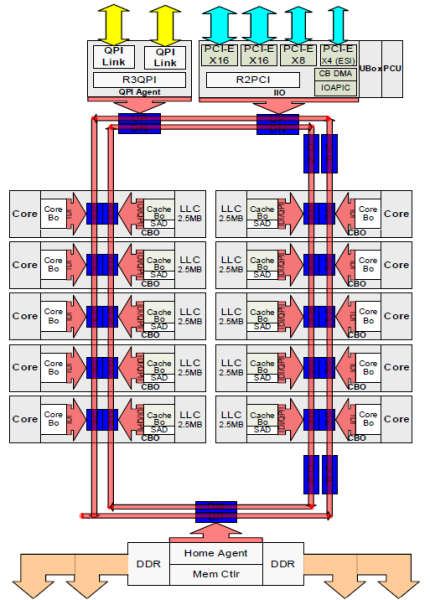
Intel provides a schematic overview of a CPU to understand the relationship between the Uncore and the cores, I’ve recreated this overview to help emphasise certain components. Please note that the following diagram depicts a High Core Count architecture of the Intel Xeon v4 (Broadwell). This is a single CPU package. The cores are spread out in a “chop-able” design, allowing Intel to offer three different core counts, Low, Medium and High. The red line is depicting the scalable on-die ring connecting the cores with the rest of the Uncore components. More in-depth information can be found in part 4 of this series.

If a CPU core wants to access data it has to communicate with the Uncore. Data can be in the last-level cache (LLC), thus interfacing with the Cbox, it might require memory from local memory, interfacing with the home agent and integrated memory controller (IMC). Or it needs to fetch memory from a remote NUMA node, as a consequence, the QPI comes into play. Due to the many components located in the Uncore, it plays a significant part in the overall power consumption of the system. With today’s focus on power reduction, the Uncore is equipped with frequency scaling functionality (UFS).

Haswell (v4) introduces Per Core Power States (PCPS) that allows each core to run at its own frequency. UFS allows the Uncore components to scale their frequency up and down independently of the cores. This allows Turbo Boost 2.0 to turbo up and owns the two elements independently, allowing cores to scale up the frequency of their LLC and ring on-ramp modules, without having to enforce all Uncore elements to turbo boost up and waste power. The feature that regulates boosting of the two elements is called Energy Efficient Turbo, some vendors provide the ability to manage power consumption with the settings Uncore Frequency Override or Uncore Frequency. These settings are geared towards applying performance savings in a more holistic way.

The Uncore provides access to all interfaces, plus it regulates the power states of the cores, therefore it has to be functional even when there is a minimal load on the CPU. To reduce overall CPU power consumption, the power control mechanism attempts to reduce the CPU frequency to a minimum by using C1E states on separate cores. If a C1E state occurs, the frequency of the Uncore is likely to be lowered as well. This could have a negative effect on the I/O throughput of the overall throughput of the CPU. To avoid this from happening some server vendors provide the BIOS option; Uncore Frequency Override. By default this option is set to Disabled, allowing the system to reduce the Uncore frequency to obtain power consumption savings. By selecting Enabled it prevents frequency scaling of the Uncore, ensuring high performance. To secure high levels of throughput of the QPI links, select the option enabled, keep in mind that this can have a negative (increased) effect on the power consumption of the system.
Some vendors provide the Uncore Frequency option of Dynamic and Maximum. When set to Dynamic, the Uncore frequency matches the frequency of the fastest core. With most server vendors, when selecting the dynamic option, the optimization of the Uncore frequency is to save power or to optimize the performance. The bias towards power saving and optimize performance is influenced by the setting of power-management policies. When the Uncore frequency option is set to maximum the frequency remains fixed.

Generally, this modularity should make it more power efficient, however, some IT teams don’t want their system to swing up and down but provide a consistent performance. Especially when the workload is active across multiple nodes in a cluster, running the workload consistently is more important that having a specific node to go as fast as it can.

Quick Path Interconnect Link

Virtual machine configuration can impact memory allocation, for example when the memory configuration consumption exceeds the available amount of local memory, ESXi allocates remote memory to this virtual machine. An imbalance of VM activity and VM resource consumption can trigger the ESXi host to rebalance the virtual machines across the NUMA nodes which lead to data migration between the two NUMA nodes. These two examples occur quite frequently, as such the performance of remote memory access, memory migration, and low-level CPU processes such as cache snooping and validation traffic depends on the QPI architecture. It is imperative when designing and configuring a system that attention must be given to the QuickPath Interconnect configuration.

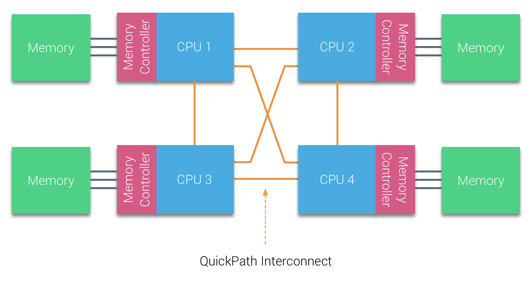
Xeon CPUs designated for dual CPU setup (E5-26xx) is equipped with two QPI bi-directional links. Depending on the CPU model selected, the QPI links operates at high frequencies measured in giga-transfers per second (GT/s). Today the majority of E5 Xeons (v4) operate at 9.6 GT/s, while some run at 6.4 GT/sec or 8.6 GT/sec. Giga-transfer per second refers to the number of operations transferring data that occur in each second in a data-transfer channel. It’s an interesting metric, however, it does not specify the bit rate. In order to calculate the data-transmission rate, the transfer rate must be multiplied by the channel width. The QPI link has the ability to transfer 16 bits of data-payload. The calculation is as follows: GT/s x channel width /bits-to-bytes.

9.6 GT/sec x 16 bits = 153.6 Bits per second / 8 = 19.2 GB/s.
The purist will argue that this is not a comprehensive calculation, as this neglects the clock rate of the QPI. The complete calculation is:
QPI clock rate x bits per Hz x channel width × duplex = bits ÷ byte. 4.8 Ghz x 2 bits/Hz x 16 x 2 / 8 = 38.4 GB/s.

Haswell (v3) and Broadwell (v4) offer three QPI clock rates, 3.2 GHz, 4.0 GHz, and 4.8 GHz. Intel does not provide clock rate details, it just provide GT/s. Therefore to simplify this calculations, just multiple GT/s by two (16 bits / 8 bits to bytes = 2). Listed as 9.6 GT/s a QPI link can transmit up to 19.2 GB/s from one CPU to another CPU. As it is bidirectional, it can receive the same amount from the other side. In total, the two 9.6 GT/s links provide a theoretical peak data bandwidth of 38.4 GB/sec in one direction.

QPI link speed	Unidirectional peak bandwidth	Total peak bandwidth
6.4 GT/s	12.8 GB/s	25.6 GB/s
8.0 GT/s	16.0 GB/s	32 GB/s
9.6 GT/s	19.2 GB/s	38.4 GB/s

There is no direct relationship with core-count and QPI link speeds. For example the v4 product family features 3 8-core count CPUs, each with a different QPI link speed, but there are also 10 core CPUs with a bandwidth of 8.0 GT/s. To understand the logic, you need to know that Intel categorizes their CPU product family into segments. Six segments exist; Basic, Standard, Advanced, Segment Optimized, Low Power and Workstation.

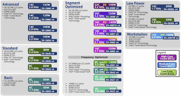
The Segment Optimized features a sub segment of Frequency Optimized, these CPU’s push the gigabit boundaries. And then off course there is the custom-build segment, which is off the list, but if you have enough money, Intel can look into your problems. The most popular CPUs used in the virtual datacenter come from the advanced and segment optimized segments. These CPUs provide enough cores and cache to drive a healthy consolidation ratio. Primarily the high core count CPUs from the Segment Optimized category are used. All CPU’s from these segments are equipped with a QPI link speed of 9.6 GT/s.

Segment	Model Number	Core count	Clock cycle	TDP	QPI speed
Advanced	E5-2650 v4	12	2.2 GHz	105W	9.6 GT/s
Advanced	E5-2660 v4	14	2.0 GHz	105W	9.6 GT/s
Advanced	E5-2680 v4	14	2.4 GHz	120W	9.6 GT/s
Advanced	E5-2690 v4	14	2.6 GHz	135W	9.6 GT/s
Optimized	E5-2683 v4	16	2.1 GHz	120W	9.6 GT/s
Optimized	E5-2695 v4	18	2.1 GHz	120W	9.6 GT/s
Optimized	E5-2697 v4	18	2.3 GHz	145W	9.6 GT/s
Optimized	E5-2697A v4	16	2.6 GHz	145W	9.6 GT/s
Optimized	E5-2698 v4	20	2.2 GHz	135W	9.6 GT/s
Optimized	E5-2699 v4	22	2.2 GHz	145W	9.6 GT/s

QPI Link Speed Impact on Performance

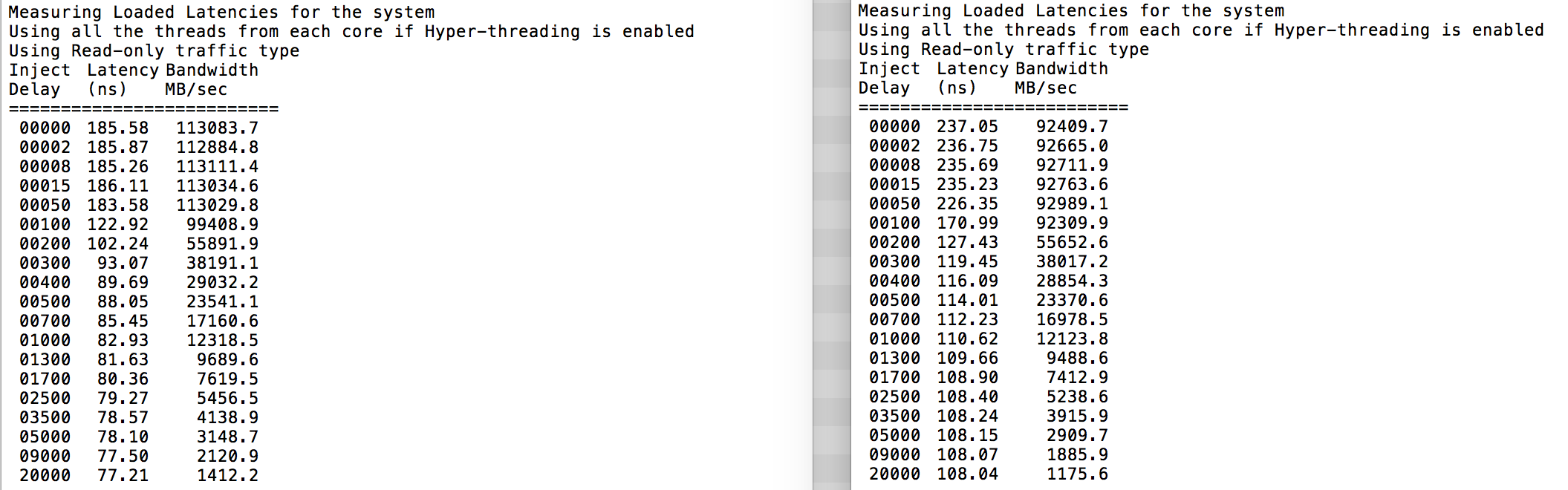
When opting for a CPU with a lower QPI link speeds, remote memory access will be impacted. During the tests of QPI bandwidth using the Intel Memory Latency Checker v3.1. it reported an average of ˜75% of the theoretical bandwidth when fetching memory from the remote NUMA node.

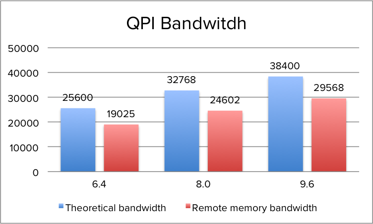
The peak bandwidth is more a theoretical maximum number as transfer data comes with protocol overhead. Additionally tracking resources are needed when using multiple links to track each data request and maintain coherency. The maximum QPI bandwidth that is available at the time of writing is lower than the minimum supported memory frequency of 1600 MHz (Intel Xeon v3 & v4). The peak bandwidth of DDR4 1600 MHz is 51 GB/s, which exceeds the theoretical bandwidth of the QPI by 32%. As such, QPI bandwidth can impact remote memory access performance. In order to obtain the most performance, it’s recommended to select a CPU with a QPI configuration of 9.6 GT/s to reduce the bandwidth loss to a minimum, the difference between 9.6 GT/s and 8.0 GT/s configuration is a 29% performance drop. AS QPI bandwidth impacts remote memory access, it’s the DIMM configuration and memory frequency that impacts local memory access. Local memory optimization is covered in Part 4.

Note!
The reason why I’m exploring nuances of power settings is that high-performance power consumption settings are not always the most optimal setting for today’s CPU microarchitecture. Turbo mode allows cores to burst to a higher clock rate if the power budget allows it. The finer details of Power management and Turbo mode are beyond the scope of this NUMA deep dive, but will be covered in the upcoming CPU Power Management Deep Dive.

Intel QPI Link Power Management

Some servers allow you to configure the QPI Link Power Management in the BIOS. When enabled, the buffers in the QPI links are allowed to enter a sleep state when the links are not being used. When there is relatively little traffic, the QPI link shuts down some of its data transmissions lanes, this to achieve power consumption reduction. Within a higher state, it only reduces bandwidth, when entering a deeper state memory access will occur latency impact.

A QPI link consists of a transmit circuit (TX), 20 data lanes, 1 clock lane and a receive circuit (RX). Every element can be progressively switched off. When the QPI is under heavy load it will use all 20 lanes, however when experiencing a workload of 40% or less it can decide to modulate to half width. Half width mode, called L0p state saves power by shutting down at least 10 lanes. The QPI power management spec allows to reduce the lanes to a quarter width, but research has shown that power savings are too small compared to modulating to 10 links. Typically when the 10 links are utilized for 80% to 90% the state shifts from L0p back to the full-width L0 state. L0p allows the system to continue to transmit data without any significant latency penalty. When no data transmit occurs, the system can invoke the L0s state. This state only operates the clock lane and its part of the physical TX and RX circuits, due to the sleep mode of the majority of circuits (lane drivers) within the transceivers no data can be sent. The last state, L1, allows the system to shut down the complete link, benefitting from the highest level of power consumption.

L0s and L1 states are costly from a performance perspective, Intel’s’ patent US 8935578 B2 indicates that exiting L1 state will cost multiple microseconds and L0s tens of nanoseconds. Idle remote memory access latency measured on 2133 MHz memory is on average 130 nanoseconds, adding 20 nanoseconds will add roughly 15% latency and that’s quite a latency penalty. A low power state with longer latency and lower power than L0s and is activated in conjunction with package C-states below C00

State	Description	Properties	Lanes
L0	Link Normal Operational State	All lanes and Forward Clock active	20
L0p	Link power saving state	A lower power state from L0 that reduces the link from full width to half width	10
L0s	Low Power Link State	Turns odd most lane drivers, rapid recovery to the L0 state	1
L0s	Deeper Low Power State	Lane drivers and Fwd clock turned off, greater power savings than L0s, Longer time to return to L0 state

If the focus is on architecting a consistent high performing platform, I recommend to disable QPI Power Management in the BIOS. Many vendors have switched their default setting from enabled to disabled, nevertheless its wise to verify this setting.

The memory subsystem and the QPI architecture lay the foundation of the NUMA architecture. Last level cache is a large part of the memory subsystem, the QPI architecture provides the interface and bandwidth between NUMA nodes. It’s the cache coherency mechanisms that play a great part in providing the ability to span virtual machines across nodes, but in turn, will impact overall performance and bandwidth consumption.
Up next, Part 3: Cache Coherency

The 2016 NUMA Deep Dive Series:
Part 0: Introduction NUMA Deep Dive Series
Part 1: From UMA to NUMA
Part 2: System Architecture
Part 3: Cache Coherency
Part 4: Local Memory Optimization
Part 5: ESXi VMkernel NUMA Constructs
Part 6: NUMA Initial Placement and Load Balancing Operations
Part 7: From NUMA to UMA

Non-uniform memory access (NUMA) is a shared memory architecture used in today’s multiprocessing systems. Each CPU is assigned its own local memory and can access memory from other CPUs in the system. Local memory access provides a low latency – high bandwidth performance. While accessing memory owned by the other CPU has higher latency and lower bandwidth performance. Modern applications and operating systems such as ESXi support NUMA by default, yet to provide the best performance, virtual machine configuration should be done with the NUMA architecture in mind. If incorrect designed, inconsequent behavior or overall performance degradation occurs for that particular virtual machine or in worst case scenario for all VMs running on that ESXi host.
This series aims to provide insights of the CPU architecture, the memory subsystem and the ESXi CPU and memory scheduler. Allowing you in creating a high performing platform that lays the foundation for the higher services and increased consolidating ratios. Before we arrive at modern compute architectures, it’s helpful to review the history of shared-memory multiprocessor architectures to understand why we are using NUMA systems today.

The evolution of shared-memory multiprocessors architecture in the last decades

It seems that an architecture called Uniform Memory Access would be a better fit when designing a consistent low latency, high bandwidth platform. Yet modern system architectures will restrict it from being truly uniform. To understand the reason behind this we need to go back in history to identify the key drivers of parallel computing.
With the introduction of relational databases in the early seventies the need for systems that could service multiple concurrent user operations and excessive data generation became mainstream. Despite the impressive rate of uniprocessor performance, multiprocessor systems were better equipped to handle this workload. In order to provide a cost-effective system, shared memory address space became the focus of research. Early on, systems using a crossbar switch were advocated, however with this design complexity scaled along with the increase of processors, which made the bus-based system more attractive. Processors in a bus system are allowed to access the entire memory space by sending requests on the bus, a very cost effective way to use the available memory as optimally as possible.

However, bus-based systems have their own scalability problems. The main issue is the limited amount of bandwidth, this restrains the number of processors the bus can accommodate. Adding CPUs to the system introduces two major areas of concern:

1. The available bandwidth per node decreases as each CPU added.
2. The bus length increases when adding more processors, thereby increasing latency.

The performance growth of CPU and specifically the speed gap between the processor and the memory performance was, and actually still is, devastating for multiprocessors. Since the memory gap between processor and memory was expected to increase, a lot of effort went into developing effective strategies to manage the memory systems. One of these strategies was adding memory cache, which introduced a multitude of challenges. Solving these challenges is still the main focus of today for CPU design teams, a lot of research is done on caching structures and sophisticated algorithms to avoid cache misses.

Introduction of caching snoop protocols

Attaching a cache to each CPU increases performance in many ways. Bringing memory closer to the CPU reduces the average memory access time and at the same time reducing the bandwidth load on the memory bus. The challenge with adding cache to each CPU in a shared memory architecture is that it allows multiple copies of a memory block to exist. This is called the cache-coherency problem. To solve this, caching snoop protocols were invented attempting to create a model that provided the correct data while not trying to eat up all the bandwidth on the bus. The most popular protocol, write invalidate, erases all other copies of data before writing the local cache. Any subsequent read of this data by other processors will detect a cache miss in their local cache and will be serviced from the cache of another CPU containing the most recently modified data. This model saved a lot of bus bandwidth and allowed for Uniform Memory Access systems to emerge in the early 1990s. Modern cache coherency protocols are covered in more detail by part 3.

Uniform Memory Access Architecture

Processors of Bus-based multiprocessors that experience the same – uniform – access time to any memory module in the system are often referred to as Uniform Memory Access (UMA) systems or Symmetric Multi-Processors (SMPs).

With UMA systems, the CPUs are connected via a system bus (Front-Side Bus) to the Northbridge. The Northbridge contains the memory controller and all communication to and from memory must pass through the Northbridge. The I/O controller, responsible for managing I/O to all devices, is connected to the Northbridge. Therefore, every I/O has to go through the Northbridge to reach the CPU.
Multiple buses and memory channels are used to double the available bandwidth and reduce the bottleneck of the Northbridge. To increase the memory bandwidth even further some systems connected external memory controllers to the Northbridge, improving bandwidth and support of more memory. However due the internal bandwidth of the Northbridge and the broadcasting nature of early snoopy cache protocols, UMA was considered to have a limited scalability. With today’s use of high-speed flash devices, pushing hundreds of thousands of IO’s per second, they were absolutely right that this architecture would not scale for future workloads.

Non-Uniform Memory Access Architecture

To improve scalability and performance three critical changes are made to the shared-memory multiprocessors architecture;

1. Non-Uniform Memory Access organization
2. Point-to-Point interconnect topology
3. Scalable cache coherence solutions

1: Non-Uniform Memory Access organization

NUMA moves away from a centralized pool of memory and introduces topological properties. By classifying memory location bases on signal path length from the processor to the memory, latency and bandwidth bottlenecks can be avoided. This is done by redesigning the whole system of processor and chipset. NUMA architectures gained popularity at the end of the 90’s when it was used on SGI supercomputers such as the Cray Origin 2000. NUMA helped to identify the location of the memory, in this case of these systems, they had to wonder which memory region in which chassis was holding the memory bits.
In the first half of the millennium decade, AMD brought NUMA to the enterprise landscape where UMA systems reigned supreme. In 2003 the AMD Opteron family was introduced, featuring integrated memory controllers with each CPU owning designated memory banks. Each CPU has now its own memory address space. A NUMA optimized operating system such as ESXi allows workload to consume memory from both memory addresses spaces while optimizing for local memory access. Let’s use an example of a two CPU system to clarify the distinction between local and remote memory access within a single system.

The memory connected to the memory controller of the CPU1 is considered to be local memory. Memory connected to another CPU socket (CPU2)is considered to be foreign or remote for CPU1. Remote memory access has additional latency overhead to local memory access, as it has to traverse an interconnect (point-to-point link) and connect to the remote memory controller. As a result of the different memory locations, this system experiences “non-uniform” memory access time.

2: Point-to-Point interconnect

AMD introduced their point-to-point connection HyperTransport with the AMD Opteron microarchitecture. Intel moved away from their dual independent bus architecture in 2007 by introducing the QuickPath Architecture in their Nehalem Processor family design.
The Nehalem architecture was a significant design change within the Intel microarchitecture and is considered the first true generation of the Intel Core series. The current Broadwell architecture is the 4th generation of the Intel Core brand (Intel Xeon E5 v4), the last paragraph contains more information on the microarchitecture generations. Within the QuickPath architecture, the memory controllers moved to the CPU and introduced the QuickPath point-to-point Interconnect (QPI) as data-links between CPUs in the system.

The Nehalem microarchitecture not only replaced the legacy front-side bus but reorganized the entire sub-system into a modular design for server CPU. This modular design was introduced as the “Uncore” and creates a building block library for caching and interconnect speeds. Removing the front-side bus improves bandwidth scalability issues, yet intra- and inter-processor communication have to be solved when dealing with enormous amounts of memory capacity and bandwidth. Both the integrated memory controller and the QuickPath Interconnects are a part of the Uncore and are Model Specific Registers (MSR) ). They connect to a MSR that provides the intra- and inter-processor communication. The modularity of the Uncore also allows Intel to offer different QPI speeds, at the time of writing the Intel Broadwell-EP microarchitecture (2016) offers 6.4 Giga-transfers per second (GT/s), 8.0 GT/s and 9.6 GT/s. Respectively providing a theoretical maximum bandwidth of 25.6 GB/s, 32 GB/s and 38.4 GB/s between the CPUs. To put this in perspective, the last used front-side bus provided 1.6 GT/s or 12.8 GB/s of platform bandwidth. When introducing Sandy Bridge Intel rebranded Uncore into System Agent, yet the term Uncore is still used in current documentation. You can find more about QuickPath and the Uncore in part 2.

3: Scalable Cache Coherence

Each core had a private path to the L3 cache. Each path consisted of a thousand wires and you can imagine this doesn’t scale well if you want to decrease the nanometer manufacturing process while also increasing the cores that want to access the cache. In order to be able to scale, the Sandy Bridge Architecture moved the L3 cache out of the Uncore and introduced the scalable ring on-die Interconnect. This allowed Intel to partition and distribute the L3 cache in equal slices. This provides higher bandwidth and associativity. Each slice is 2.5 MB and one slice is associated with each core. The ring allows each core to access every other slice as well. Pictured below is the die configuration of a Low Core Count (LCC) Xeon CPU of the Broadwell Microarchitecture (v4) (2016).

This caching architecture requires a snooping protocol that incorporates both distributed local cache as well as the other processors in the system to ensure cache coherency. With the addition of more cores in the system, the amount of snoop traffic grows, since each core has its own steady stream of cache misses. This affects the consumption of the QPI links and last level caches, requiring ongoing development in snoop coherency protocols. An in-depth view of the Uncore, scalable ring on-Die Interconnect and the importance of caching snoop protocols on NUMA performance will be included in part 3.

Non-interleaved enabled NUMA = SUMA

Physical memory is distributed across the motherboard, however, the system can provide a single memory address space by interleaving the memory between the two NUMA nodes. This is called Node-interleaving (setting is covered in part 2). When node interleaving is enabled, the system becomes a Sufficiently Uniform Memory Architecture (SUMA). Instead of relaying the topology info and nature of the processors and memory in the system to the operating system, the system breaks down the entire memory range into 4KB addressable regions and maps them in a round robin fashion from each node. This provides an ‘interleaved’ memory structure where the memory address space is distributed across the nodes. When ESXi assigns memory to virtual machine it allocates physical memory located from two different nodes when the physical CPU located in Node 0 needs to fetch the memory from Node 1, the memory will traverse the QPI links.

The interesting thing is that the SUMA system provides a uniform memory access time. Only not the most optimal one and heavily depends on contention levels in the QPI architecture. Intel Memory Latency Checker was used to demonstrate the differences between NUMA and SUMA configuration on the same system.
This test measures the idle latencies (in nanoseconds) from each socket to the other socket in the system. The latency reported of Memory Node 0 by Socket 0 is local memory access, memory access from socket 0 of memory node 1 is remote memory access in the system configured as NUMA.

NUMA	Memory Node 0	Memory Node 1	–	SUMA	Memory Node 0	Memory Node 1
Socket 0	75.7	132.0	–	Socket 0	105.5	106.4
Socket 1	131.9	75.8	–	Socket 1	106.0	104.6

As expected interleaving is impacted by constant traversing the QPI links. The idle memory test is the best case scenario, a more interesting test is measuring loaded latencies. It would have been a bad investment if your ESXi servers are idling, therefor you can assume that an ESXi system is processing data. Measuring loaded latencies provides a better insight on how the system will perform under normal load. During the test the load injection delays are automatically changed every 2 seconds and both the bandwidth and the corresponding latency is measured at that level. This test uses 100% read traffic.NUMA test results on the left, SUMA test results on the right.

The reported bandwidth for the SUMA system is lower while maintaining a higher latency than the system configured as NUMA. Therefore, the focus should be on optimizing the VM size to leverage the NUMA characteristics of the system.

Nehalem & Core microarchitecture overview

With the introduction of the Nehalem microarchitecture in 2008, Intel moved away from the Netburst architecture. The Nehalem microarchitecture introduced Intel customers to NUMA. Along the years Intel introduced new microarchitectures and optimizations, according to its famous Tick-Tock model. With every Tick, optimization takes place, shrinking the process technology and with every Tock a new microarchitecture is introduced. Even though Intel provides a consistent branding model since 2012, people tend to Intel architecture codenames to discuss the CPU tick and tock generations. Even the EVC baselines lists these internal Intel codenames, both branding names and architecture codenames will be used throughout this series:

Microarchitecture DP servers	Branding	Year	Cores	LLC (MB)	QPI Speed (GT/s)	Memory Frequency	Architectural change	Fabrication Process
Nehalem	x55xx	10-2008	4	8	6.4	3xDDR3-1333	Tock	45nm
Westmere	x56xx	01-2010	6	12	6.4	3xDDR3-1333	Tick	32nm
Sandy Bridge	E5-26xx v1	03-2012	8	20	8.0	4xDDR3-1600	Tock	32nm
Ivy Bridge	E5-26xx v2	09-2013	12	30	8.0	4xDDR3-1866	Tick	22 nm
Haswell	E5-26xx v3	09-2014	18	45	9.6	4xDDR3-2133	Tock	22nm
Broadwell	E5-26xx v4	03-2016	22	55	9.6	4xDDR3-2400	Tick	14 nm

Up next, Part 2: System Architecture
The 2016 NUMA Deep Dive Series:
Part 0: Introduction NUMA Deep Dive Series
Part 1: From UMA to NUMA
Part 2: System Architecture
Part 3: Cache Coherency
Part 4: Local Memory Optimization
Part 5: ESXi VMkernel NUMA Constructs

Recently I’ve been analyzing traffic to my site and it appears that a lot CPU and memory articles are still very popular. Even my first article about NUMA published in february 2010 is still in high demand. And although you see a lot of talk about the upper levels and overlay technology today, the focus on proper host design and management remains. After all, it’s the correct selection and configuration of these physical components that produces a consistent high performing platform. And it’s this platform that lays the foundation for the higher services and increased consolidating ratios.

Most of my NUMA content published throughout the years is still applicable to the modern datacenter, yet I believe the content should be refreshed and expanded with the advancements that are made in the software and hardware layers since 2009.

To avoid ambiguity, this deep dive is geared towards configuring and deploying dual socket systems using recent Intel Xeon server processors. After analyzing the dataset of more than 25.000 ESXi host configurations collected from virtual datacenters worldwide, we discovered that more than 80% of ESXi host configuration are dual socket systems. Today, according to IDC, Intel controls 99 percent of the server chip market.
Despite the strong focus of this series on the Xeon E5 processor in a dual socket setup, the VMkernel, and VM content is applicable to systems running AMD processors or multiprocessor systems. No additional research was done on AMD hardware configurations or performance impact when using high-density CPU configurations.

The 2016 NUMA Deep Dive Series

The 2016 NUMA Deep Dive Series consists of 7 parts.The 2016 NUMA deep dive series is split into three main categories; Physical, VMkernel, and Virtual Machine.

Part 1: From UMA to NUMA
Part 1 covers the history of multi-processor system design and clarifies why modern NUMA systems cannot behave as UMA systems anymore.

Part 2: System Architecture
The system architecture part covers the Intel Xeon microarchitecture and zooms in on the Uncore. Primarily focusing on Uncore frequency management and QPI design decisions.

Part 3: Cache Coherency
The unsung hero of today’s NUMA architecture. Part 3 zooms in to cache coherency protocols and the importance of selection the proper snoop mode.

Part 4: Local Memory Optimization
Memory density impacts the overall performance of the NUMA system, part 4 dives into the intricacy of channel balance and DIMM per Channel configuration.

Part 5: ESXi VMkernel NUMA Constructs
The VMkernel has to distribute the virtual machines to provide the best performance. This part explores the NUMA constructs that are subject to initial placement and load-balancing operations.

Part 6: NUMA Initial Placement and Load Balancing Operations
The VMkernel has to distribute the virtual machines to provide the best performance. This part explores the NUMA initial placement and load-balancing operations. (not yet released)

Part 7: From NUMA to UMA
The world of IT moves in loops of iteration, the last 15 years we moved from UMA to NUMA systems, which today’s focus on latency and the looming licensing pressure, some forward-thinking architects are looking into creating high performing UMA systems. (not yet released)

The articles will be published on a daily basis to avoid saturation. Similar to other deep dives, the articles are lengthy and contain lots of detail. Up next, Part 1: From UMA to NUMA