Introduction
We are amid the AI “gold rush.” More organizations are looking to incorporate any form of machine learning (ML) or deep learning in their services to enhance customer experience, drive efficiencies in their processes or improve quality of life (healthcare, transportation, smart cities).
Train Where Data is Generated
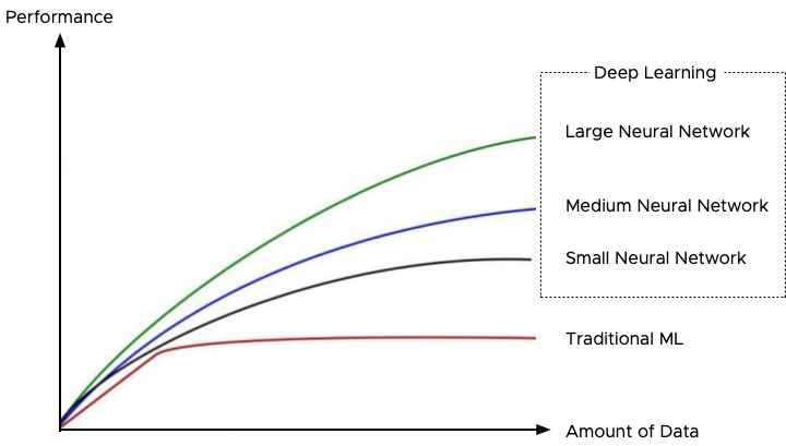
One of the key elements that drive on-premise ML focused infrastructure growth is the reality of data gravity. Mentioned in the article “Multi-GPU and Distributed Deep Learning,” deep learning (DL) gets better with data. Consequently, data sets used for ML and DL training purposes are growing at a tremendous rate. These vast data sets need to be processed. Data transit, hosting, and the necessary compute cycles impact the overall OPEX budget. Additionally, data protection regulations such as data residency, data sovereignty, and data locality impact where data can be stored outside the place it is created. As a result, a lot of forward-leaning organizations are repatriating their AI platforms to run ML and DL workloads close to the systems that generate the data.
And what better platform to run ML and DL workloads than vSphere? Machine learning comes with its own set of lingo, and different personas interacting with the machine learning stack. To be able to have a meaningful conversation with data scientists and ML engineers, you need to have a basic understanding of how each component interacts with each other. You don’t have to learn the ins and out of the different neural networks, but having an idea of what a particular component does help you understand how it might impact your service levels and your selection of components of the vSphere platform used for ML workloads.
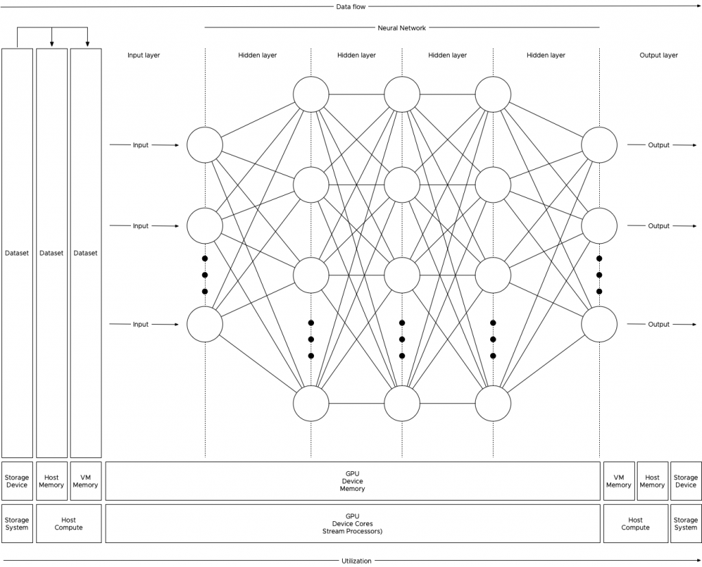
To give an example, OpenCL and Vulkan are frameworks that allow for the execution of code on GPU (General Purpose GPU). Using this framework allows you to theoretically expose any GPUs to a machine learning framework such as Tensorflow or Pytorch. As it’s open-source, you can use it on all kinds of GPUs from different vendors. However, all popular actively-developed frameworks do not support OpenCL or Vulkan and only use the NVIDIA CUDA API framework, thus impacting your hardware selection for the vSphere host design. I created an overview of the different layers of the deep learning technology stack, attempting to make sense of the relationships between the components of each different layer.
Deep Learning Technology Stack

Let’s use a bottom-up approach for reviewing the deep learning technology stack.
vSphere Constructs and Accelerators
Hardware over the last 20 years looked uniform, other than the vendor and some minor vendor-specific functionality; the devices appeared relatively similar to a guest OS. Most code can run on an AMD as well as an Intel without changing. Hardware competed on scale and speed, not on different ways how it can interact with software. Today’s acceleration devices are very diverse and expose their explicit architecture to the application. The hardware specifics determine the code and algorithm used in the application. And therefore, we need to expose these devices to the application in its most raw and unique form. As a result, the overview primarily covers acceleration devices such as GPUs and FPGAs.
However, recently Rice University released a new research paper called: “SLIDE: In Defense of Smart Algorithms over Hardware Acceleration for Large-Scale Deep Learning Systems“. They are demonstrating that by using a fundamentally different approach, it is possible to accelerate deep learning without using hardware accelerators like GPUs.
Our evaluations on industry-scale recommendation datasets, with large fully connected architectures, show that training with SLIDE on a 44 core CPU is more than 3.5 times (1-hour vs. 3.5 hours) faster than the same network trained using TF on Tesla V100 at any given accuracy level. On the same CPU hardware, SLIDE is over 10x faster than TF
I assume the authors meant a dual-socket system with two 22-cores Xeon CPUs, but an exciting development that certainly needs to be closely followed. For now, let’s concentrate on the components used by the majority of the deep-learning community.
vSphere can expose the accelerator devices via two constructs right now, DirectPath I/O (Passthrough) and NVIDIA vGPU. In 2020 two additional constructs will be available; Dynamic DirectPath I/O (information will follow soon) and Bitfusion. Bitfusion pools and shares accelerators across VMs inside the cluster. It provides virtual remote attached GPUs that can be shared between VMs fully or fractionally. Bitfusion can even assign multiple GPUs to a single VM to support any form of distributed deep learning strategy.
DirectPath I/O
DirectPath I/O, often called Passthrough, provides similar functionality as bare-metal GPU. DirectPath I/O is used for maximum hardware device performance inside the VM and to use native vendor driver and app stack support in the guest OS and the application. Perfect for running specialized software libraries provided by the CUDA stack, which is covered in a later paragraph. DirectPath I/O allows for maximum performance because the I/O mapped from the application and guest OS directly to the hardware device; the VMkernel (Hypervisor) is not involved.
A complete device is assigned to a single VM and cannot be shared with other active VMs. This prohibits fractional use of the device (i.e., assigning half of the device resources to a VM). DirectPath I/O allows assigning multiple GPUs to a VM.
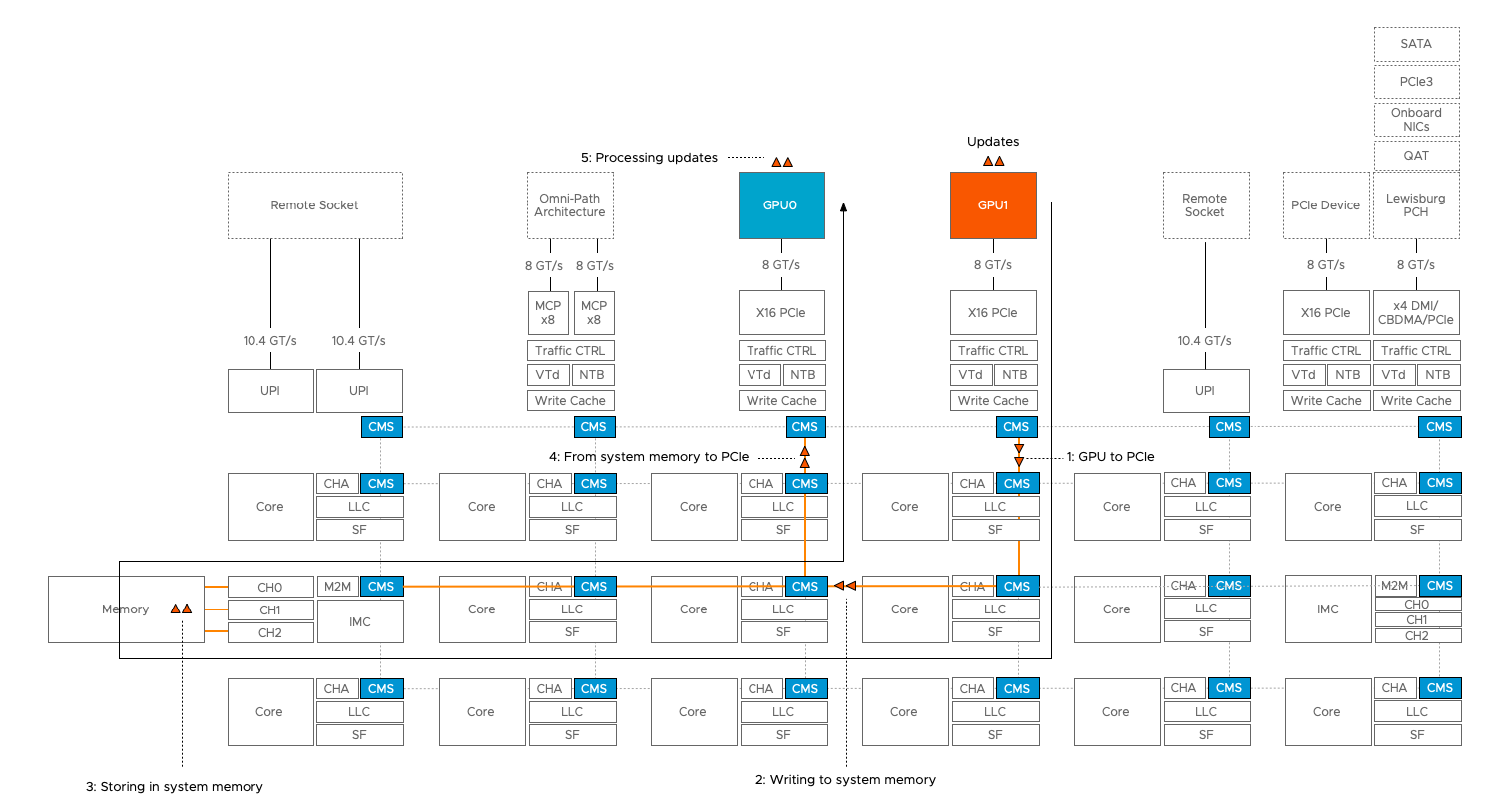
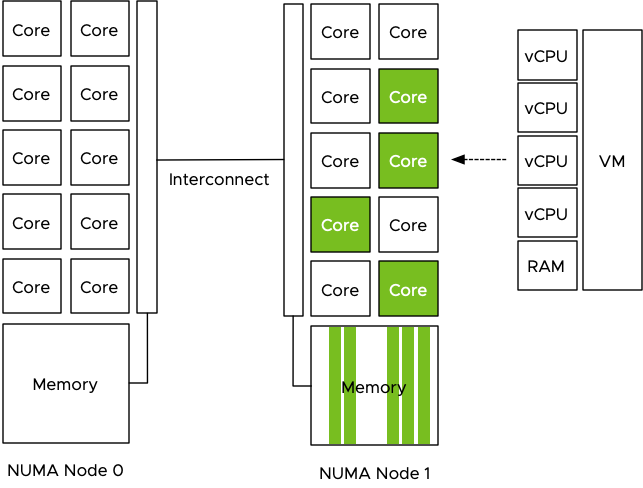
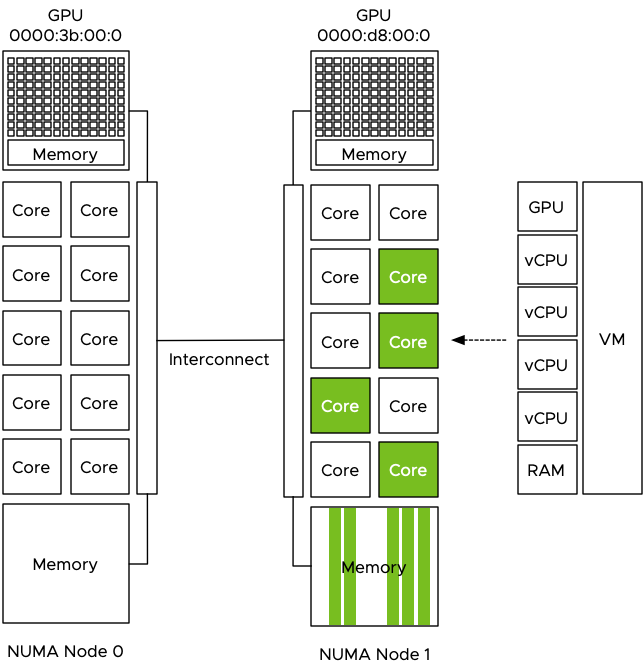
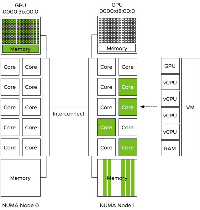
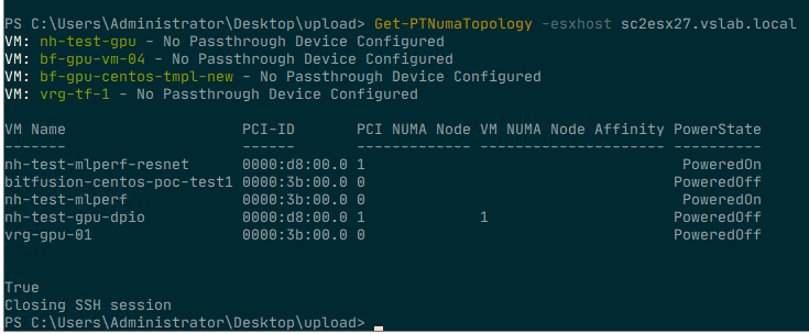
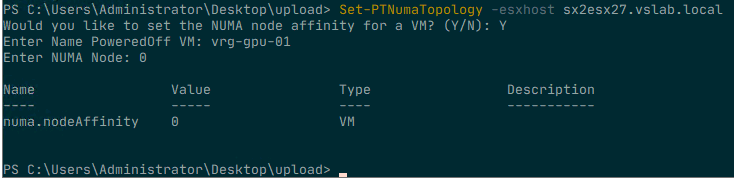
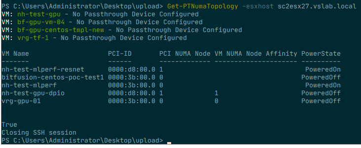
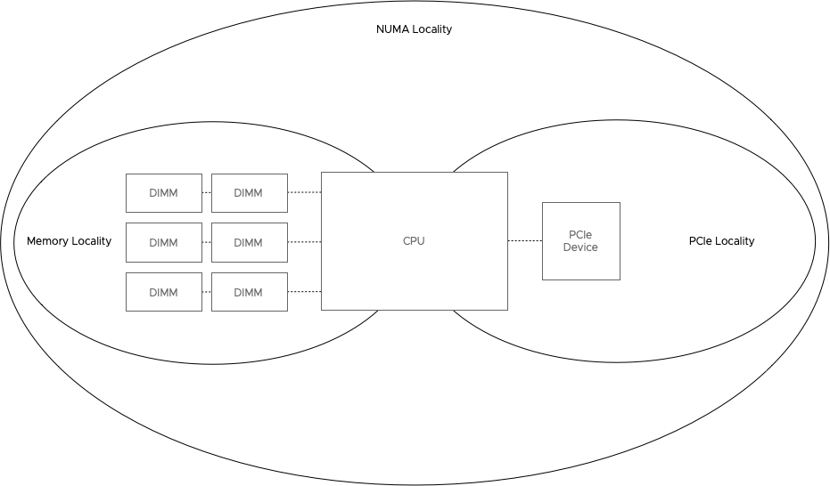
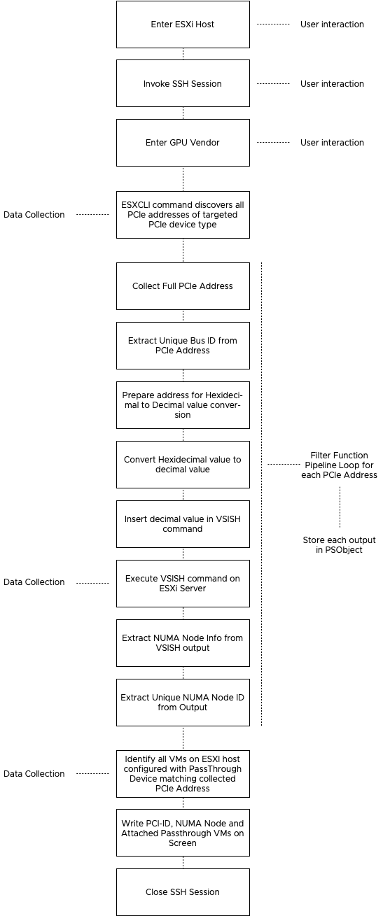
When a DirectPath I/O device is assigned to a virtual machine, it uses the physical location of the device for the assignment, i.e., Host:Bus: Device-Physical-Function. (The article “Machine Learning Workload and GPGPU NUMA Node Locality” describes locality assignment in detail). Due to this, DirectPath I/O is not compatible with certain core virtualization features, such as vMotion (and thus DRS).
Design Impact
Currently, vSphere does not support the AMD Radeon Server Accelerators for Deep learning (Radeon Instinct). vSphere supports only NVIDIA GPUs at the moment. From vSphere 6.7 update 1, FPGAs can also be directly exposed to the guest OS by using DirectPath I/O. At the time of writing this article, vSphere 6.7 update 1 supports the Intel Arria 10 GX FPGA. More details on the vSphere blog.
NVIDIA vGPU
NVIDIA virtual GPU (vGPU) provides advanced GPU virtualization functionality that enables the sharing of GPU devices across VMs. An NVIDIA GPU can be logically partitioned (fractional GPU) to multiple virtual GPUs. A VM can use multiple vGPUs that are located in the same host. Both the hypervisor and the VM need to run NVIDIA software to provide fractional, full, and multiple vGPU functionalities.

Bitfusion
In 2019, VMware acquired Bitfusion, and I’m looking forward to having this functionality available to our customers. Bitfusion FlexDirect software allows for pooling GPU resources and providing a dynamic remote attach service. That means that workload can run on vSphere hosts that do not have GPU hardware installed. The beauty of this solution is that it does not require any changes to the application. It uses native CUDA (see acceleration libraries paragraph) to intercept the application calls, the FlexDirect software sends it to the FlexDirect server across the network. The Flexdirect server has a DirectPath I/O connection to all the GPUs in that host and manages the placement and scheduling of the workloads.
This model corresponds heavily to the early days of virtualization. We used to have 1000’s x86 servers in the data center, each having an average utilization of less than 10% while costing a lot of money. We consolidated compute resources and managed the workload in such a manner than peak utilization did not overlap. With the rise of general-purpose computing on GPU, we see the same patterns. The GPUs are not cheap, sometimes the cost of a GPU server is an order of magnitude more expensive than a “traditional” server. However, when we look at the utilization, we see an average usage of 5 to 20%.
Deep Learning Development Cycle
With deep-learning, you cannot just pump some data into a deep-learning model and expect a result. The data scientist has to gather training data, asses the data quality. The next step is to choose an algorithm and a framework. Often the data is not formatted correctly for the used model. The data set needs to be improved; typically, data scientists need to deal with outliers and extreme values, missing or inaccurate data. Data for supervised learning needs to be labeled, and the data set needs to be split up into training data sets and evaluation data sets. Now the deep-learning can begin, and the GPU is fed the data. The deep learning framework executes the model. After a single epoch, the data scientist reviews the effectiveness of the model and possibly adjust the model to improve prediction. The model is trained again to verify if the adjustments are correct. Once the model behaves appropriately, it deployed to production where it can run inference tasks that generate predictions based on new data. Each step consuming a lot of time, however only two moments (marked in red) utilize the expensive GPU hardware. Creating the problem, interestingly called “dark silicon”.

It doesn’t make sense to keep those resource isolated and assigned to a VM that can only be used by a specific data scientist. By introducing remote virtualization, a GPU can be shared between many different virtual machines. A Bitfusion server can contain multiple GPUs, and many Bitfusion servers can be active on the network. Abstracting the hardware and allow for remote execution of API calls, creates a solution that is easily scaled out. Orchestrating workload placement ensures that a pool of GPUs can be made available to the data scientist when the model is ready for training.

During the Tech Field Day, Mazhar Memom (CTO Bitfusion) covered the Bitfusion architecture, showing the use of CUDA libraries by the application to interact with the GPU device. In Bitfusion’s case, it is sending these remote API calls to a server that controls the hardware. But this brings us to the statement made earlier in the article. We have arrived at a time in which the software depends heavily on abstraction layers. In the AI space, it is no different. A deep learning model is going to use a framework that uses a set of libraries that are provided by the hardware vendor. This model allows the application developer to quickly (and correctly) to consume the hardware functionality to drive application performance. The defacto toolkit for the deep learning ecosystem is NVIDIA’s Compute Unified Device Architecture (CUDA). The next article covers the subsequent layers in the DL framework stack in more depth.