• Skip to primary navigation
  • Skip to main content

frankdenneman.nl

  • AI/ML
  • NUMA
  • About Me
  • Privacy Policy

Solving vNUMA Topology Mismatch When Migrating between Dual Socket Servers and Quad Socket Servers

March 11, 2022 by frankdenneman

I recently received a few questions from customers migrating between clusters with different CPU socket footprints. The challenge is not necessarily migrating live workloads between clusters because we have Enhanced vMotion Compatibility (EVC) to solve this problem. 

For VMware users just learning about this technology, EVC masks certain unique features of newer CPU generations and creates a generic baseline of CPU features throughout the cluster. If workloads move between two clusters, vMotion still checks whether the same CPU features are presented to the virtual machine. If you are planning to move workloads, ensure the EVC modes of the clusters are matching to get the smoothest experience.

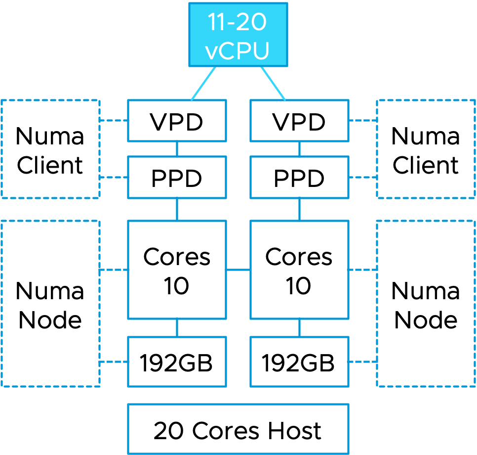
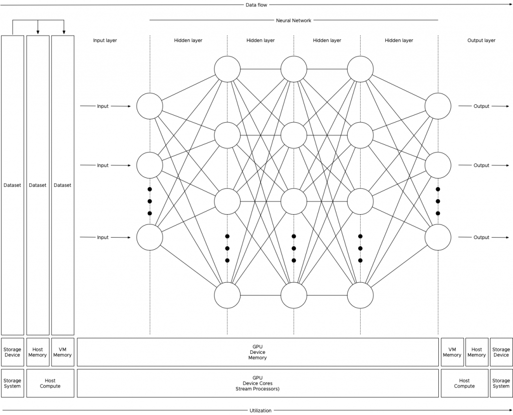
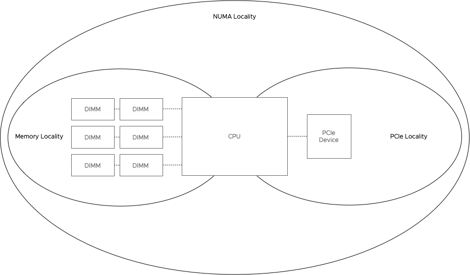
The challenge when moving live workloads between ESXi hosts with different socket configurations is that vNUMA topology of the virtual machine does not match the physical topology. A virtual NUMA topology exists out of two components, the component that presents the CPU topology to the virtual machine, called the VPD. The VPD exists to help the guest OS and the applications optimize their CPU scheduling decisions. This VPD construct is principally the virtual NUMA topology. The other component, the PPD, groups the vCPUs and helps the NUMA scheduler for placement decisions across the physical NUMA nodes.

The fascinating part of this story is that the VPD and PPD are closely linked, yet they can differ if needed. The scheduler attempts to mirror the configuration between the two elements; the PPD configuration is dynamic, but the VPD configuration always remains the same. From the moment the VM is powered on, the VPD configuration does not change. And that is a good thing because operating systems generally do not like to see whole CPU layouts change. Adding a core with CPU hot add is all right. But drastically rearranging caches and socket configurations it’s pretty much a bridge too far. 

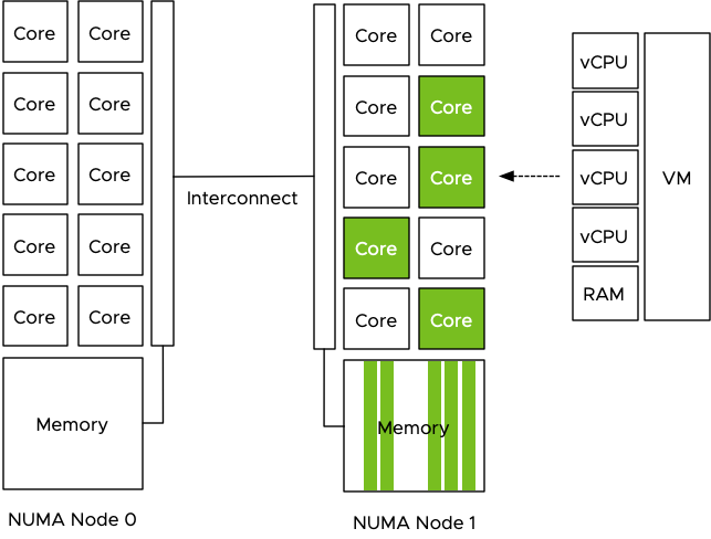
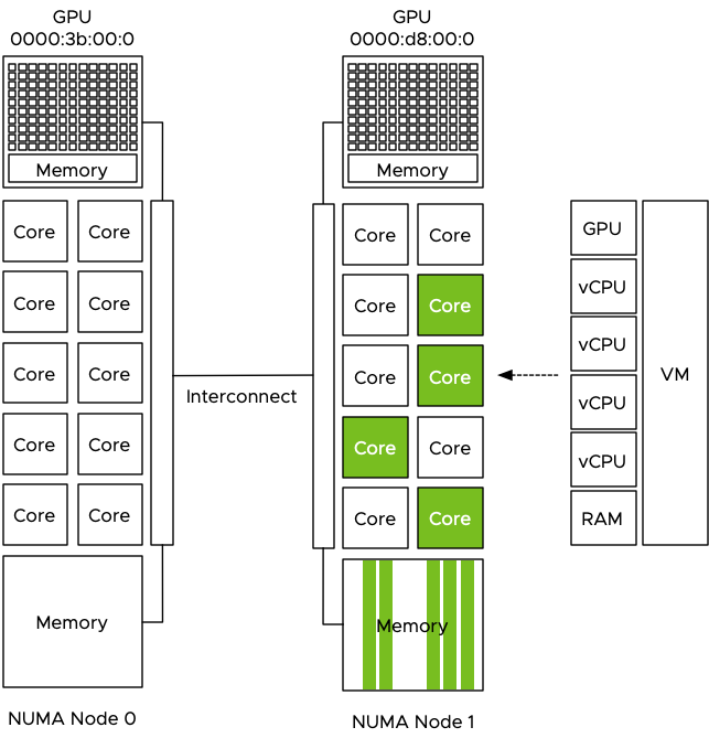
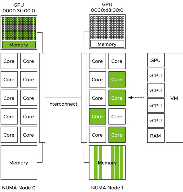
As mentioned before, the VPD remains the same. Still, the NUMA scheduler can reconfigure the PPD to optimize the vCPU grouping for the CPU scheduler. When will this happen? When you move a VM to a host with a different physical CPU configuration, i.e. Socket Count, or physical cores per socket count. This way, ESXi still squeezes out the best performance it can in this situation. The drawback of this situation is the mismatch between presentation and scheduling.

This functionality is great as it allows workloads to enjoy mobility between different CPU topologies without any downtime. However, we might want to squeeze out all the performance possible. Some vCPUs might not share the same cache, although the application thinks they do. Or, some vCPU might not even be scheduled together in the same physical NUMA node, experiencing latency and bandwidth reduction. To be more precise, this mismatch can impact memory locality and the action-affinity load-balancing operations of the scheduler. Thus, it can impact the VM performance and create more inter CPU traffic. This impact might be minor on a per-VM basis, but you have to think in scale, the combined performance loss of all the VMs, so for larger environments, it might be worthwhile to get it fixed.

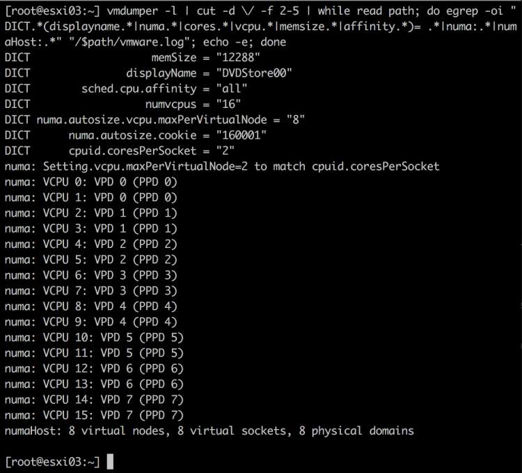
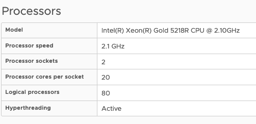
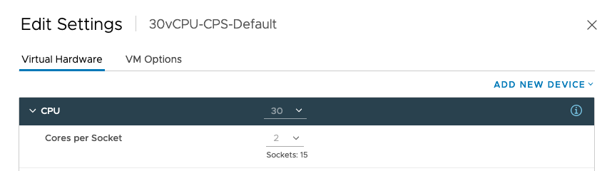
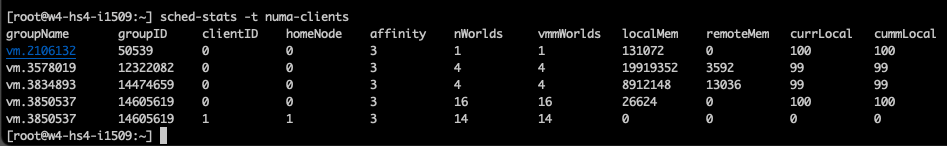
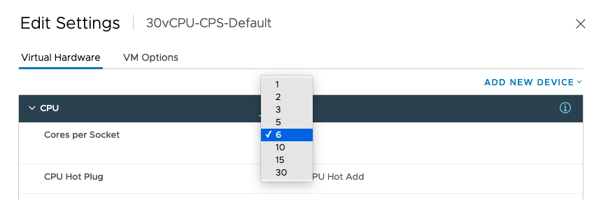
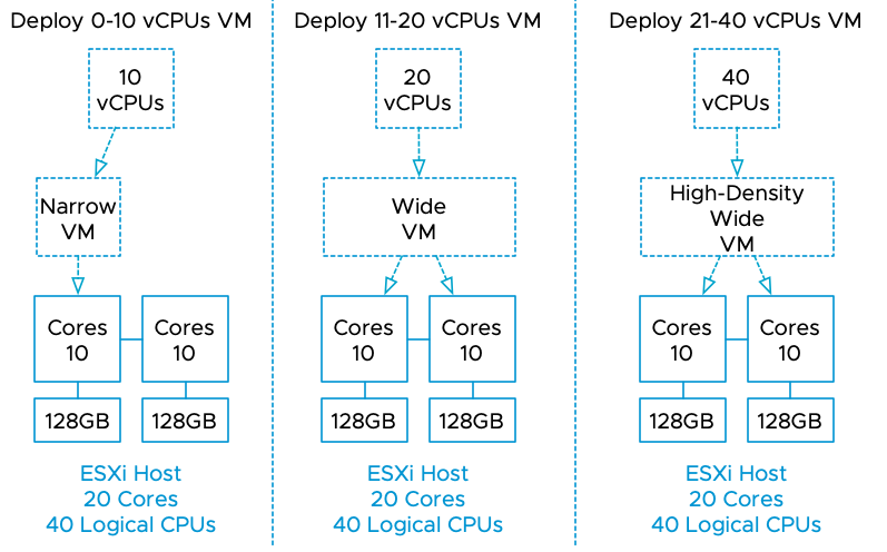
I’ve created a 36 vCPU VM on a dual-socket system with twenty physical CPU cores per socket. The power-on process of the virtual machine creates the vNUMA topology and enters all kinds of entries in the VMX file. Once the VM powers on, the VMX file receives the following entries.

numa.autosize.cookie = "360022"
numa.autosize.vcpu.maxPerVirtualNode = "18"

The key entry for this example is the “numa.autosize.vcpu.maxPerVirtualNode = “18”, as the NUMA scheduler likes to distribute as many vCPUs across many cores as possible and evenly across sockets. 

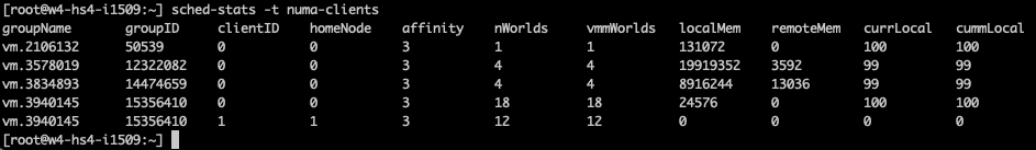
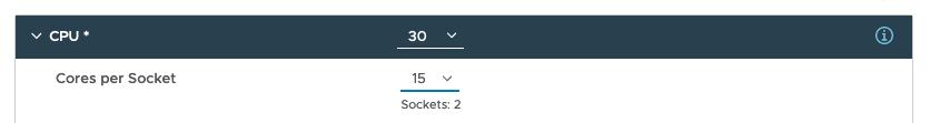
But what happens if this virtual machine moves to a quad-socket system with 14 physical cores per socket? The NUMA scheduler will create three scheduling constructs to distribute those vCPUs across the NUMA nodes but keep the presentation layer the same not to confuse the guest OS and the applications.

Since the NUMA topologies are created during a VM’s power-on, we have to shut down the virtual machine and power it back to realign the VPD and PPD topology again. Well, since 2019, we don’t need to power down the VM anymore! And I have to admit. I only found out about it just recently. Bob Plankers (not this Bob) writes about the vmx.reboot.PowerCycle advanced parameter here. This setting does not require a complete power cycle anymore. 

That means that if you are in the process of migrating your VM estate from dual-socket systems to quad-socket systems, you can add the following adjustments in the VMX file while the VM is running. (for example via PowerCLI / New-AdvancedSetting)

vmx.reboot.PowerCycle = true
numa.autosize.once = false

The setting vmx.reboot.PowerCycle will remove itself from the VMX file, but it’s best to remove the numa.autosize.once = false from the VMX file. So you might want to track this. Same as adding the setting, you can remove the setting while the VM is up and running.

When you have applied these settings to the VMX, the next time the VM reboots, the vNUMA topology will be changed. As always, keep in mind that older systems might react more dramatically than newer systems. After all, you are changing the hardware topology of the system. It might upset an older windows system or optimizations of an older application. Some older operating systems do not like this and will need to do reconfiguration themselves or need some help from the IT ops team. In the worst-case scenario, it will treat the customer to a BSOD with that in mind. It’s recommended to work with the customer with old OSes and figure out a test and migration plan.

Special thanks to Gilles Le Ridou for helping me confirm my suspicion and helping me test scenarios on his environment. #vCommunity!

Filed Under: NUMA

vSphere 7 Cores per Socket and Virtual NUMA

December 2, 2021 by frankdenneman

Regularly I meet with customers to discuss NUMA technology, and one of the topics that are always on the list is the Cores per Socket setting and its potential impact.

In vSphere 6.5, we made some significant adjustments to the scheduler that allowed us to decouple the NUMA client creation from the Cores per Socket setting. Before 6.5, if the vAdmin configured the VM with a non-default Cores per Socket setting, the NUMA scheduler automatically aligned the NUMA client configured to that Cores per Socket settings. Regardless of whether this configuration was optimal for performing in its physical surroundings.

To help understand the impact of this behavior, we need to look at the components of the NUMA client and how this impacts the NUMA scheduler options for initial placement and load-balancing options.

A NUMA client consists of two elements, a virtual component and a physical component. The virtual component is called the virtual proximity domain (VPD) and is used to expose the virtual NUMA topology to the guest OS in the virtual machine, so the Operating System and its applications can apply optimizations for the NUMA topology they detect. The physical component is called the physical proximity domain (PPD). It is used by the NUMA scheduler in the VMkernel as a grouping construct for vCPUs to place a group of vCPUs on a NUMA node (physical CPU+memory) and to move that group of vCPUs between NUMA nodes for load-balancing purposes. You can see this PPD as some form of an affinity group. These vCPUs always stick together.

Please note that the CPU scheduler determines which vCPU will be scheduled on a CPU core. The NUMA scheduler only selects the NUMA node.

As depicted in the diagram, this VM runs on a dual-socket ESXi host. Each CPU socket contains a CPU package with 10 CPU cores. If this VM gets configured with a vCPU range between 11 and 20 vCPUs, the NUMA scheduler creates two NUMA clients and distributes these vCPUs evenly across the two NUMA nodes. The guest OS is presented with a virtual NUMA topology by the VPDs that aligns with the physical layout. In other words, there will be two NUMA nodes, with an x number of CPUs inside that NUMA node.

Previous to ESXi 6.5, if a virtual machine is created with 16 CPUs and 2 Cores per Socket, the NUMA scheduler will create 8 NUMA Clients, and thus the VM exposes eight NUMA nodes to the guest OS.

As a result, the guest OS and application could make the wrong process placement decisions or miss out on ideal optimizations as you are reducing resource domains as memory ranges and cache domains. Luckily we solved this behavior, and now the Cores Per Socket setting does not influence NUMA client configuration anymore. But!

But, a Cores per Socket setting other than Cores per Socket =1 will impact the distribution of vCPUs of that virtual machine across the physical NUMA nodes. As the Cores per Socket act as a mini affinity rule-set. That means that the NUMA schedule has to distribute the vCPUs of the virtual machine across the NUMA nodes with Cores per Settings still in mind, not as drastically as before, where it also exposed it to the guest OS. Still, it will impact overall balance if you start to do weird things. Let me show you some examples. Let’s start by using a typical example of Windows 2019. In my lab, I have a dual-socket Xeon system with each 20 cores, so I’m forced to equip the example VMs with more than 20 vCPUs to show you the effect of Cores per Socket on vNUMA.

In the first example, I deploy a Windows 2019 VM with the default settings and 30 vCPUs. That means that it is configured with 2 Cores per Socket. Resulting in a virtual machine configuration with 15 sockets.

The effect is seen by using the command “sched-stats -t numa-clients” if I log into the ESXi host via an SSH session. The groupID of the VM is 1405619, which I got from ESXTOP, and this command shows that 16 vCPUs are running on homeNode 0 and 14 vCPUs on homeNode 1. Maybe, this should not be a problem, but I’ve seen things! Horrible things!

This time I’ve selected 6 Cores per socket. And now the NUMA scheduler distributes the vCPUs as follows:

At this point, the NUMA nodes are imbalanced more severely. This will impact the guest OS and the application. And If you do this at scale, for every VM in your DC, you will create a scenario where you impact the guest OS and the underlying fabric of connected devices. More NUMA rebalancing is expected, which occurs across the processor interconnects (QPI-Infinity Fabric). More remote memory is fetched, all the operations impact PCIe traffic, networking traffic, HCI storage traffic, GPU VDI or Machine Learning application performance.

The Cores per Socket setting is invented to solve a licensing problem. There are small performance gains to be made if the application is sensitive to cache performance and can keep the data in the physical cache. If you have that application, please align your Cores per Socket setting to the actual physical layout. Using the last example, for the 30 vCPU VM on a dual-socket 40 cores host, the Cores per Socket should be 15, resulting in 2 virtual sockets.

But my recommendation is to avoid the management overhead for 99% of all your workload and keep the default Cores per Socket Settings. Overall you have a higher chance not to impact any underlying fabric or influence scheduler decisions.

Update

Looking at the comments, I notice that there is some confusion. Keeping the default means that you will use 2 Cores per Socket for the new Windows systems. The minor imbalance of vCPU distribution within the VM should not be noticeable. The Windows OS is smart enough to distribute processes efficiently between these NUMA nodes setup like this. The compounded effect of many VMs within the hypervisor and the load-balancing mechanism of the NUMA scheduler and the overall load frequencies (not every vCPU is active all of the time) will not make this a problem.

For AMD EPYC users, please keep in mind, that you are not working with a single chip surface anymore. EPYC is a multi-chip module architecture and hence, you should take notice of the cache boundaries of the CCX’s within the EPYCs. The new Milan (v3) has 8 cores per CCX, the Rome (v2) and Naples (v1) have 4 cores. Please test the cache boundary sensitivity of your workload if you are running your workload on AMD EPYC systems. Please note that not every workload is cache sensitive and not every combination of workloads responds the same way. This is due to the effect that load correlation and load synchronicity patterns can have on scheduling behavior and cache evictions patterns.

Filed Under: NUMA

VM Service – Help Developers by Aligning Their Kubernetes Nodes to the Physical Infrastructure

May 3, 2021 by frankdenneman

The vSphere 7.0 U2a update released on April 27th introduces the new VM service and VM operator. Hidden away in what seems to be a trivial update is a collection of all-new functionalities. Myles Gray has written an extensive article about the new features. I want to highlight the administrative controls of VM classes of the VM service.

VM Classes
What are VM classes, and how are they used? With Tanzu Kubernetes Grid Service running in the Supervisor cluster, developers can deploy Kubernetes clusters without the help of the Infra Ops team. Using their native tooling, they specify the size of the cluster control plane and worker nodes by using a specific VM class. The VM class configuration acts a template used to define CPU, memory resources and possibly reservations for these resources. These templates allow the InfraOps team to set guardrails for the consumption of cluster resources by these TKG clusters.

The supervisor cluster provides twelve predefined VM classes. They are derived from popular VM sizes used in the Kubernetes space. Two types of VM classes are provided, a best-effort class and a guaranteed class. The guaranteed class edition fully reserves its configured resources. That is, for a cluster, the spec.policies.resources.requests match the spec.hardware settings. A best-effort class edition does not, that is, it allows resources to be overcommitted. Let’s take a closer look at the default VM classes.

VM Class TypeCPU ReservationMemory Reservation
Best-Effort-‘size’0 MHz0 GB
Guaranteed-‘size’Equal to CPU configEqual to memory config

There are eight default sizes available for both VM class types. All VM classes are configured with a 16GB disk.

VM Class SizeCPU Resources ConfigurationMemory Resources Configuration
XSmall22 Gi
Small24 Gi
Medium28 Gi
Large416 Gi
XLarge432 Gi
2 XLarge16128 Gi
4 XLarge16128 Gi
8 XLarge32128 Gi

Burstable Class
One of the first things you might notice if you are familiar with Kubernetes is that the default setup is missing a QoS class, the Burstable kind. Guaranteed and Best-Effort classes are located at both ends of the spectrum of reserved resources (all or nothing). The burstable class can be anywhere in the middle. I.e., the VM class applies a reservation for memory and or CPU. Typically, the burstable class is portrayed to be a lower-cost option for workloads that do not have a sustained high resource usage. Still, I think the class can play an essential role in no-chargeback cloud deployments.

To add burstable classes to the Supervisor Cluster, go to the Workload Management view, select the Services tab, and click on the manage option of the VM Service. Click on the “Create VM Class” option and enter the appropriate settings. In the example below, I entered 60% reservations for both CPU and memory resources, but you can set independent values for those resources. Interestingly enough, no disk size configuration is possible.

Although the VM Class is created, you have to add it to a namespace to be made available for self-service deployments.

Click on “Add VM Class” in the VM Service tile. I modified the view by clicking on the vCPU column, to find the different “small” VM classes and selected the three available classes.

After selecting the appropriate classes, click ok. The Namespace Summary overview shows that the namespace offers three VM classes.

The developer can view the VM classes assigned to the namespace by using the following command:

kubectl get virtualmachineclassbindings.vmoperator.vmware.com -n namespacename I logged into the API server of the supervisor cluster, changed the context to the namespace “onlinebankapp” and executed the command:

kubectl get virtualmachineclassbindings.vmoperator.vmware.com -n onlinebankapp

If you would have used the command “kubectl get virtualmachineclass -n onlinebankapp“, you get presented with the list of virtualmachineclasses available within the cluster.

Help Developers by Aligning Their Kubernetes Nodes to the Physical Infrastructure

With the new VM service and the customizable VM classes, you can help the developer align their nodes to the infrastructure. Infrastructure details are not always visible at the Kubernetes layers, and maybe not all developers are keen to learn about the intricacies of your environment. The VM service allows you to publish only the VM classes you see fit for that particular application project. One of the reasons could be the avoidance of monster-VM deployment. Before this update, developers could have deployed a six worker node Kubernetes cluster using the guaranteed 8XLarge class (each worker node equipped with 32 vCPUs, 128Gi all reserved), granted if your hosts config is sufficient. But the restriction is only one angle to this situation. Long-lived relationships are typically symbiotic of nature, and powerplays typically don’t help build relationships between developers and the InfraOps team. What would be better is to align it with the NUMA configuration of the ESXi hosts within the cluster.

NUMA Alignment
I’ve published many articles on NUMA, but here is a short overview of the various NUMA configuration of VMs. If a virtual machine (VM) powers on, the NUMA scheduler creates one or more NUMA clients based on the VM CPU count and the physical NUMA topology of the ESXi host. For example, a VM with ten vCPUs powered on an ESXi host with ten cores per NUMA node (CPN2) is configured with a single NUMA client to maximize resource locality. This configuration is a narrow-VM configuration. Because all vCPU have access to the same localized memory pool, this can be considered an Unified Memory Architecture (UMA).

Take the example of a VM with twelve vCPUs powered-on on the same host. The NUMA scheduler assigns two NUMA clients to this VM. The NUMA scheduler places both NUMA clients on different NUMA nodes, and each NUMA client contains six vCPUs to distribute the workload equally. This configuration is a wide VM configuration. If simultaneous multithreading (SMT) is enabled, a VM can have as many vCPUs equal to the number of logical CPUs within a system. The NUMA scheduler distributes the vCPUs across the available NUMA nodes and trusts the CPU scheduler to allocate the required resources. A 24 vCPU VM would be configured with two NUMA clients, each containing 12 vCPUs if deployed on a 10 CPN2 host. This configuration is a high-density wide VM.

A great use of VM service is to create a new set of VM classes aligned with the various NUMA configurations. Using the dual ten core system as an example, I would create the following VM classes and the associated CPU and memory resource reservations :

CPUMemoryBest EffortBurstableBurstable Mem OptimizedGuaranteed
UMA-Small216GB0% | 0%50% | 50%50% | 75%100% | 100%
UMA-Medium432GB0% | 0%50% | 50%50% | 75%100% | 100%
UMA-Large648GB0% | 0%50% | 50%50% | 75%100% | 100%
UMA-XLarge864GB0% | 0%50% | 50%50% | 75%100% | 100%
NUMA-Small1296GB0% | 0%50% | 50%50% | 75%100% | 100%
NUMA-Medium14128GB0% | 0%50% | 50%50% | 75%100% | 100%
NUMA-Large16160GB0% | 0%50% | 50%50% | 75%100% | 100%
NUMA-XLarge18196GB0% | 0%50% | 50%50% | 75%100% | 100%

The advantage of curating VM classes is that you can align the Kubernetes nodes with a physical NUMA node’s boundaries at CPU level AND memory level. In the table above, I create four classes that remain within a NUMA node’s boundaries and allow the system to breathe. Instead of maxing out the vCPU count to what’s possible, I allowed for some headroom, avoiding a noisy neighbor with a single NUMA node and system-wide. Similar to memory capacity configuration, the UMA-sized (narrow-VM) classes have a memory configuration that does not exceed the physical NUMA boundary of 128GB, increasing the chance that the ESXi system can allocate memory from the local address range. The developer can now query the available VM classes and select the appropriate VM class with his or her knowledge about the application resource access patterns. Are you deploying a low-latency memory application with a moderate CPU footprint? Maybe a UMA-Medium or UMA-large VM class helps to get the best performance. The custom VM class can transition the selection process from just a numbers game (how many vCPUs do I want?) to a more functional requirement exploration (How does it behave?) Of course, these are just examples, and these are not official VMware endorsements.

In addition, I created a new class, “Burstable mem optimized”, A class that reserves 25% more memory capacity than its sibling VM class “Burstable”. This could be useful for memory-bound applications that require the majority of memory to be reserved to provide consistent performance but do not require all of it. The beauty of custom VM classes is that you can design them as they fit your environment and your workload. With your skillset and knowledge about the infrastructure, you can help the developer to become more successful.

Filed Under: Kubernetes, NUMA

Machine Learning Workload and GPGPU NUMA Node Locality

January 30, 2020 by frankdenneman

In the previous article “PCIe Device NUMA Node Locality” I covered the physical connection between the processor and the PCIe device briefly touched upon machine learning workloads with regards to PCIe NUMA locality. This article zooms in on why it is important to consider PCIe NUMA locality.

General-Purpose Computing on Graphics Processing Units

New compute-intensive workloads take advantage of the new programming model called general-purpose computing on GPU (GPGPU). With GPGPU, the many cores integrated on modern GPUs are used to offload a vast number of (parallel) compute threads from the CPU. By adding another computational device with different characteristics, a heterogeneous compute architecture is born. GPUs are optimized for streaming sequential (or easily predictable) access patterns, while CPUs are designed for general access patterns and concurrency of threads. Combined, they form a GPGPU pipeline, that is exceptionally well-suited to analyze data. The vSphere platform is well-suited to create GPGPU pipelines and optimizations are provided to VMs, such as DirectPath I/O Access (also known as Passthrough). Passthrough allows the application to interface with the accelerator device directly; however, data must be transferred from disk/network through the system (RAM) to the GPU. And controlling the data transfer is of interest to the overall performance of the platform for both GPGPU workload and non-GPGPU workload.

A very popular GPGPU workload is Machine Learning (ML). Many ML workloads process gigabytes of data, sometimes even terabytes, this data flows from the storage device up to the PCIe device. Finetuning the configuration and placement of the virtual machine running the ML workload can benefit the data-scientist and other consumers of the platform. Not every ML workload is latency-sensitive, but most data scientists prefer to get the training done as quickly as possible. This allows them to perform more training iterations to fine-tune the model (also known as the neural network). Due to the movement of data through the system, a ML workload can quickly become the noisiest neighbor you ever saw in your system. But with the right guard-rails in place, data-scientists take advantage of running their workload on a consistent performing platform, while the rest of the organization can consume resources from this platform as well.

Machine Learning Concepts

Oversimplified ML is “using data to answer questions.” With traditional programming models, you create “rules” by using the programming language and apply these rules to the input to get output (results) (output). With ML training, you provide input and the output to train the program to create rules. This creates a predictive model that can be used to analyze previously unseen data to provide accurate answers. The key component of the entire ML process is data. This data is stored on a storage device and fetched to be used as input for the model to be trained on, or to use the trained model to provide results. Training a machine learning model is primarily done by a neural network of nodes that are executed by thousands of cores on GPUs. The nature of the cores (SIMT – Single Instruction, Multiple Data) allows for extremely fast parallel processing, ideal for this sort of workload, hence you want to use GPUs for this task and not the serial-workload optimized CPUs. The heavy lifting of the compute part is done by the GPU, but the challenge is getting the data to the costly GPU cores as fast and consistent as possible. If you do not keep the GPU cores fed with all the data it needs, then a large part of the GPU cores sit idle until new data shows up. And this is the challenge to overcome, handling large quantities of training data that flows from storage, through the host memory, into the VM memory before flowing into the memory of the GPU. High-speed storage systems with fast caching and fast paths between the storage, CPU, server memory and PCIe device are necessary.

Anatomy of an ML Training Workload

The collection of training examples is called a dataset, and the golden rule is, the more data you can use during the training, the better the predictive model becomes. That means that the data scientist will unleash copious amounts of data on the system, data so large that it cannot fit inside the memory device of the GPU. Perhaps not even the memory assigned to the virtual machine, as a result, the data is stored on disk and is retrieved in batches. 

The data scientist typically finetunes the size of the batch set, finetuning a batch set size is considered an art form in the world of ML. You, the virtual admin, slowly graduating into an ML infrastructure engineer (managing and help to design the ML platform), can help inform the data scientist by sizing the virtual machine correctly. Look at CPU consumption and determine the correct number of vCPUs necessary to push the workload. Once the GPU receives a batch, the workload is contained within the GPU. Rightsizing the VM can help to improve performance further as the VM might fit a single NUMA node.

To understand the dataflow of an ML workload through the system, let’s get familiar with some neural network terminology. Most of the ML workload use the Compute Unified Device Architecture (CUDA) for GPU programming, and when using a batch of the training data, the CUDA program takes the following steps:

1: Allocate space on the GPU device memory

2: Copy (batch set) input data to the device (aka Host to Device (HtoD))

3: Run the algorithm on the GPU cores

4: Copy output (results) back to host memory (aka Device to Host (DtoH))

During training, the program processes all the training examples in the dataset. This cycle is called an epoch. As mentioned before, a data scientist can decide to split up the entire dataset into smaller batch sets. The number of training examples used is called a batch size. An iteration is the number of passes the program needs to use to go through the entire dataset to complete a single epoch. For example, a dataset contains 100.000 samples, and each batch size contains 1000 training examples, then it takes 100 iterations to complete a single epoch. Each iteration uses the previously described CUDA loop. To get a better result, multiple epochs are pushed to get a better convergence of the training model. Within each epoch, the neural network self-tweaks its own parameters (called weights and is done for each node) in the neural network, this finetuning provides a more accurate prediction result when it’s used during the inference operation. The interesting part is that the data scientist can also make some adjustments to the (hyper)parameters of the ML model. Simply put, a hyperparameter is a parameter whose value is set before the training process begins. Such as the number of weights or the batch size set. To verify if this tuning was helpful, a new sequence of epochs is kicked off. A great series of videos about neural networks can be found here.

Josh Simons and Justin Murray gave a 4-hour workshop on ML workload on vSphere at VMworld last year. In this workshop, they stated that the typical values they saw were gigabytes of data (D), 10 to 100s of epochs (E), and 10 or more tuning cycles (T), which can be substantially more (in the 1000s) when researching new models. You can imagine that such data volumes can become a challenge in a shared system such as the hypervisor. Let’s take a look at why isolation can benefit both ML workload and the other resident workload on the system.

CPU Scheduler and NUMA optimizations

When the data is fetched from the storage device it is stored in memory. The compute schedulers of the VMkernel are optimized to store the memory as close to the CPUs as possible. Let’s use the most popular server configuration in today’s data center, the dual-socket system. Each socket contains a processor and within the processor, memory controllers exist. Memory modules (DIMMs) attached to these memory controllers are considered local memory capacity. Both processors are connected to each other to allow each processor to access the memory connected to the other processor. Due to the difference in latency and bandwidth, this is considered to be non-uniform memory access (NUMA). For more information about NUMA, check out this series.

Let use the example of a 4 vCPU VM with 32 GB, running on a host with 512GB memory with 2 processors containing 10 cores each. The dataset used is 160GB of data and it cannot be stored in the VM memory and in the GPU device memory, thus the data scientist sets the batch size to 16GB. The program fetches 16GB of training data from the datastore and the NUMA scheduler ensures the data is stored within the local memory of the processor the four vCPU run on. In this case, the vCPUs of the VM are scheduled on the cores of CPU 1 (NUMA node 1) and thus the NUMA scheduler requests the VMkernel memory scheduler to store it in the memory pages belonging to the memory address space managed by the memory controllers of CPU 1.

The VM is configured with a passthrough GPU and the training data is pushed to the GPU. The problem is that the GPU is manually selected by the admin and no direct relation is visible in the UI or command-line, it just shows the type name and a PCI address. GPUs are PCIe devices and they are hardwired and controlled by a CPU.

The admin selected the first GPU in the list and now the dataset is pushed directly from the VM memory to the GPU Device memory to be used by the cores of the GPU. Data now flows through the interconnect to the PCIe controller of CPU 0 and to the GPU device. Each dataset that is retrieved from storage, is stored in NUMA node 1 and then moved through the interconnect to the device, this is done for each iteration, for each epoch and this can be done 1000’s of time.

The problem is that the interconnect is used by the entire system. When the CPU needs to rebalance, it can reschedule the vCPU on cores belonging to a different CPU if this improves the overall resource availability for the active virtual machines. Memory can be transferred over to the new NUMA home node of that recently migrated virtual machine, or memory is just accessed across the interconnect. Same with Wide-VMs, VMs that span multiple NUMA nodes, it can happen that these Wide-VMs access a lot of “remote” memory. Also do not forget the data being handled by other PCIe devices. All network traffic has to flow from the NIC to a particular VM, for optimized performance, the kernel prefers to store that data in memory that is local to the vCPUs of that VM. The same goes for data coming from external storage devices, if the HBA or NIC is “hanging” off the other CPU, data has to flow through the interconnect. The interconnect is a highway shared by a lot of components and workloads. These operations can impact the performance of the ML workload but the opposite is also true, pushing 1000 epochs of gigabytes of data to a GPU ensures other workloads will notice the presence of that workload, even if it has a small CPU and memory footprint. Remember, ML is “using data to answer questions.”

PTNumaTopology PowerCLI Module

To make sense of it all, I created a simple PowerCLI module with two functions that show the VMs that have a passthrough device configured. The output shows the VM name and the PCI address of the device so that you can relate that to what you see in the UI. The next column shows the NUMA node to which the PCIe device is connected. The next column indicates whether the advanced setting numa.affinity is set for that particular VM and its value. The last column shows the power state of the VM. To set the NUMA affinity, the VM has to be powered off.

To run the script, import the module (available at GitHub) and execute the Get-PTNumaTopology command. Specify the FQDN of the ESXi host. For example: Get-PTNumaTopology -esxhost sc2esx27.vslab.local. As the script needs to execute a command on the ESXi host locally an SSH session is initiated. This results in a prompt for a (root) username and password in a separate login screen. (The Github page has a thorough walk-through of all the steps involved and a list of requirements.)

NUMA Affinity Advanced Setting

In most situations, it is not recommended to set any affinity setting as it simply restricts the scheduler to generate an optimal balance between resource providers (CPUs) and consumers (vCPUs). At the host level and cluster level. However since the VM is configured with a passthrough (PT) GPU, it cannot move to another host and chances are a lot of data will flow to this device. Another assumption is that the host contains a small number of GPUs and thus a small number of VMs are active. If no other restrictions are configured, the CPU and NUMA scheduler can try to work “around” the affined VM and attempt to optimize the placement and resource consumptions of the other active VMs. Hopefully, the isolation of these particular passthrough-enabled VMs are reducing overall system load and thus evening out the possible enforced restrictions. Testing this first before using it on the production workload is always recommended! For more information about the NUMA affinity setting, please consult the VMware Docs for your specific vSphere version, linked is the VMware Docs page for vSphere 6.7.

Why set numa.affinity and not use CPU pinning? First of all, CPU pinning is something that should not be done ever. And even when you think you have a valid use case, chances are that CPU pinning will still reduce performance significantly. This topic is rearing its ugly head again and I will soon post another article why CPU pinning is just a bad idea. NUMA affinity creates a rule for the CPU scheduler to find a CPU core or HT within the boundaries of the CPU itself. In the example of the 4 vCPU running on the 10 core CPU. Let’s say hyperthreading is enabled, it allows the CPU scheduler to schedule one of these four CPUs on the 20 available logical processors. If the system is not over-utilized, it can use a complete core for a vCPU, it can find the optimal placement for that workload and for the others using the same CPU. With pinning you restrict the vCPUs to only run on that particular logical processor. If chosen incorrectly you might have just selected HTs only.

If you decide to set a NUMA affinity on a particular VM, the Get-PTNumaTopology function can help you to set it correctly. As a failsafe, the script proceeds to ask if you would like to set the NUMA node affinity of a powered off VM. Answer “N” to end the script and return to the command-line. If you answer “Y” for yes, it will then ask you to provide the name of the VM. Please note that this setting can only be applied on a powered-off VM. Setting an advanced setting means that the system is writing to this to the VMX file and the VMX file is in a locked state during the power-on state of a VM. The next step is to provide the NUMA Node you want the vCPUs to set the affinity for. Use the same number listed in the PCI NUMA Node column behind the attached passthrough device.

Once the advanced setting is configurated it shows the configured value. To verify whether the setting matches the NUMA node of the passthrough device, run the command Get-PTNumaTopology again. As it has closed the SSH connection after the last run, you are required to log in again with the root user account to retrieve the current settings.

Setting the NUMA node advanced option for a VM is something that should be done for specific reasons, do not use the script for all your virtual machines. The NUMA affinity setting applies to the placement of vCPU only. The NUMA scheduler provides recommendations to the memory scheduler, but it is up to the memory scheduler discretion to store the data. The kernel is optimized to keep the memory close to the vCPUs as possible, but sometimes it cannot fit that memory into that node. Either because the VM configuration exceeds the total capacity of that node, or that other active VMs are already using large amounts of memory of that node. Setting the affinity is not a 100% guarantee that all the resources are local, but in the majority of use-cases, it will. Isolating the workload within a specific NUMA node will help to provide you consistent performance and will reduce a lot of interconnect bandwidth consumption. Enjoy using the script!

Font used in PowerShell environment: JetBrains Mono – available at – https://www.jetbrains.com/lp/mono/#intro

Filed Under: AI & ML, CPU, NUMA Tagged With: GPGPU, GPU, Machine Learning, NUMA, PCIe, VMware, vSphere

PCIe Device NUMA Node Locality

January 10, 2020 by frankdenneman

During this Christmas break, I wanted to learn PowerCLI properly. As I’m researching the use-cases of new hardware types and workloads in the data center, I managed to produce a script to identify the PCIe Device to NUMA Node Locality within a VMware ESXi Host. The script set contains a script for the most popular PCIe Device types for data centers that can be assigned as a passthrough device. The current script set is available on Github and contains scripts for GPUs, NICs and (Intel) FPGAs.

PCIe Devices Becoming the Primary Units of Data Processing

Due to the character of new workloads, the PCIe device is quickly moving up from “just” being a peripheral device to become the primary unit for data processing. Two great examples of this development are the rise of General Purpose GPU (GPGPU), often referred to as GPU Compute, and the virtualization of the telecommunication space.

The concept of GPU computing implies using GPUs and CPUs together. In many new workloads, the processes of an application are executed on a few CPU cores, while the GPU, with its many cores, handles the computational intensive data-processing part. Another workload, or better said, a whole industry that leans heavily on the performance of PCIe devices, is the telecommunication industry. Virtual Network Functions (VNF) require platforms using SR-IOV capable NICs or SmartNICs to provide ultra-fast packet processing performance.

In both scenarios having insight into PCIe Device to processor locality is a must to provide the best performance to the application or avoid introducing menacing noisy neighbors that can influence the performance of other workloads active in the system.

PCIe Device NUMA Node Locality

The majority of servers used in VMware virtualized environments are two CPU socket systems. Each CPU socket accommodates a processor containing several CPU cores. A processor contains multiple memory controllers offering a connection to directly connected memory. An interconnect (Intel: QuickPath Interconnect (QPI) & UltraPath Interconnect (UPI), AMD: Infinity Fabric (IF)) connects the two processors and allows the cores within each processor to access the memory connected to the other processor. When accessing memory connected directly to the processor, it is called local memory access. When accessing memory connected to the other processor, it is called remote memory access. This architecture provides Non-Uniform Memory Access (NUMA) as access latency, and bandwidth differs between local memory access or remote memory access. Henceforth these systems are referred to as NUMA systems.

It was big news when the AMD Opteron and Intel Nehalem Processor integrated the memory controller within the processor. But what about PCIe devices in such a system? Since the Sandy Bridge Architecture (2009), Intel reorganized the functions critical to the core and grouped them in the Uncore, which is a “construct” that is integrated into the processor as well. And it is this Uncore that handles the PCIe bus functions. It provides access to NVMe devices, GPUs, and NICs. Below is a schematic overview of a 28 core Intel Sky lake processor showing the PCIe ports and their own PCIe root stack.

Intel Skylake Mesh Architecture

In essence, a PCIe device is hardwired to a particular port on a processor. And that means that we can introduce another concept to NUMA locality, which is PCIe locality. Considering PCIe locality when scheduling low-latency or GPU compute workload can be beneficial not only to the performance of the application itself but also to the other workloads active on the system.

NUMA Locality Venn Diagram

For example, Machine Learning involves processing a lot of data, and this data flows within the system from the CPU and memory subsystem to the GPU to be processed. Properly written Machine Learning application routines minimize communication between the GPU and CPU once the dataset is loaded on the GPU, but getting the data onto the GPU typically turns the application into a noisy neighbor to the rest of the system. Imagine if the GPU card is connected to NUMA node 0, and the application is running on cores located in NUMA node 1. All that data has to go through the interconnect to the GPU card.

The interconnect provides more theoretical bandwidth than a single PCIe 3.0 device can operate at, ~40 GB/s vs. 15 GB/s. But we have to understand that interconnect is used for all PCIe connectivity and memory transfers by the CPU scheduler. If you want to explore this topic more, I recommend reviewing Amdahl’s Law – Validity of the single processor approach to achieving large scale computing capabilities – published in 1967. (Still very relevant) And the strongly related Little’s Law. Keeping the application processes and data-processing software components on the same NUMA node keeps the workloads from flooding the QPI/UPI/ AMD IF interconnect.

For VNF workloads, it is essential to avoid any latency introduced by the system. Concepts like VT-d (Virtualization Technology for Directed I/O) reduces the time spent in a system for IOs and isolate the path so that no other workload can affect its operation. Ensuring the vCPU operates within the same NUMA domain ensures that no additional penalties are introduced by traffic on the interconnect and ensures the shortest path is provided from the CPU to the PCIe device.

Constraining CPU Placement

The PCIe Device NUMA Node Locality script assists in obtaining the best possible performance by identifying the PCIe locality of GPU, NIC of FPGA PCIe devices within VMware ESXi hosts. Typically VMs running NFV or GPGPU workloads are configured with a PCI passthrough enabled device. As a result, these VMware PowerCLI scripts inform the user which VMs are attached directly to the particular PCIe devices.

Currently, the VMkernel schedulers do no provide any automatic placement based on PCIe locality. CPU placement can be controlled by associating the listed virtual machines with a specific NUMA node using an advanced setting.

Please note that applying this setting can interfere with the ability of the ESXi NUMA scheduler to rebalance virtual machines across NUMA nodes for fairness. Specify NUMA node affinity only after you consider the rebalancing issues.

The Script Set

The purpose of these scripts is to identify the PCIe Device to NUMA Node locality within a VMware ESXi Host. The script set contains a script for the most popular PCIe Device types for Datacenters that can be assigned as a passthrough device. The current script set contains scripts for GPUs, NICs, and (Intel) FPGAs.

Please note that these scripts only collect information and do not alter any configuration in any way possible.

Requirements

  • VMware PowerCLI
  • Connection to VMware vCenter
  • Unrestricted Script Execution Policy
  • Posh-SSH
  • Root Access to ESXi hosts

Please note that Posh-SSH only works on Windows version of PowerShell.

The VMware PowerCLI script primarily interfaces with the virtual infrastructure via a connection to the VMware vCenter Server. A connection (Connect-VIServer) with the proper level of certificates must be in place before executing these scripts. The script does not initiate any connect session itself. It assumes this is already in-place.

As the script extracts information from the VMkernel Sys Info Shell (VSI Shell) the script uses Posh-SSH to log into ESXi host of choice and extracts the data from the VSI Shell for further processing. The Posh-SSH module needs to be installed before running the PCIe-NUMA-Locality scripts, the script does not install Posh-SSH itself. This module can be installed by running the following command Install-Module -Name Posh-SSH (Admin rights required). More information can be found at https://github.com/darkoperator/Posh-SSH

Root access is required to execute a vanish command via the SSH session. It might be possible to use SUDO, but this has functionality has not been included in the script (yet). The script uses Posh-SSH keyboard-interactive authentication method and presents a screen that allows you to enter your root credentials securely.

Script Content

Each script consists of three stages, Host selection & logon, data collection, and data modeling. The script uses the module Posh-SSH to create an SSH connection and runs a vsish command directly on the node itself. Due to this behavior, the script creates an output per server and cannot invoke at the cluster level.

Host Selection & Logon

The script requires you to enter the FQDN of the ESXi Host, and since you are already providing input via the keyboard, the script initiates the SSH session to the host, requiring you to login with the root user account of the host. When using the GPU script, the input of the GPU vendor name is requested. The input can be, for example, NVIDIA, AMD, Intel, or any other vendor providing supported GPU devices. This input is not case-sensitive.

Data Collection

The script initiates an esxcli command that collects the PCIe address of the chosen PCIe device type. It stores the PCIe addresses in a simple array.

Data Modeling

The NUMA node information of the PCIe device is available in the VSI Shell. However, it is listed under the decimal value of the Bus ID of the PCIe address of the device. The part that follows is a collection of instructions converting the full address space into a double-digit decimal value. Once this address is available, it’s inserted in a VSISH command and execute on the ESXi host via the already opened SSH connection. The NUMA node, plus some other information, is returned by the host, and this data is trimmed to get the core value and store it in a PSobject. Throughout all the steps of the data modeling phase, each output of the used filter functions is stored in a PSObject. This object can be retrieved to verify if the translation process was executed correctly. Call $bdfOutput to retrieve the most recent conversion. (as the data of each GPU flows serially through the function pipeline, only the last device conversion can be retrieved by calling $bdfOutput.

The next step is to identify if any virtual machines registered on the selected host are configured with PCIe passthrough devices corresponding with the discovered PCIe addresses.

Output

A selection of data points is generated as output by the script:

PCIe
Device
Output Values
GPUPCI ID, NUMA Node, Passthrough Attached VMs
NICVMNIC name, PCI ID, NUMA Node, Passthrough Attached VMs
FPGAPCI ID, NUMA Node, Passthrough Attached VMs

The reason why the PCI ID address is displayed is that when you create a VM, the vCenter UI displays the (unique) PCI-ID first to identify the correct card. An FPGA and GPU do not have a VMkernel label, such as the VMNIC label of a network card. No additional information about the VMs is provided, such as CPU scheduling locations or vNUMA topology, as these are expensive calls to make and can change every CPU Quorum (50 ms).

It’s recommended to review the CPU topology of the virtual machine and if possible to set the NUMA Node affinity following the instructions listed in VMware Resource Management Guide. Please note that using this advanced setting can impact the ability of the CPU and NUMA schedulers to achieve an optimal balance.

Using the Script Set

  • Step 1. Download the script by clicking the “Download” button on the Github repository
  • Step 2. Unlock scripts (Properties .ps1 file, General tab, select Unlock.)
  • Step 3. Open PowerCLI session.
  • Step 4. Connect to VIServer
  • Step 5. Execute script for example, the GPU script: .\PCIE-NUMA-Locality-GPU.ps1
  • Step 6. Enter ESXi Host Name
  • Step 7. Enter GPU Vendor Name
  • Step 8. Enter Root credentials to establish SSH session

Step 8. Consume output and possibly set NUMA Node affinity for VMs

Acknowledgments

This script set would not have been created without the guidance of @kmruddy and @lucdekens. Thanks, Valentin Bondzio, for verification of NUMA details and Niels Hagoort and the vSphere TM team for making their lab available to me.

Filed Under: NUMA, VMware

  • « Go to Previous Page
  • Page 1
  • Page 2
  • Page 3
  • Page 4
  • Interim pages omitted …
  • Page 6
  • Go to Next Page »

Copyright © 2025 · SquareOne Theme on Genesis Framework · WordPress · Log in