• Skip to primary navigation
  • Skip to main content

frankdenneman.nl

  • AI/ML
  • NUMA
  • About Me
  • Privacy Policy

Sapphire Rapids Memory Configuration

February 28, 2023 by frankdenneman

The 4th generation of the Intel Xeon Scalable Processors (codenamed Sapphire Rapids) was released early this year, and I’ve been trying to wrap my head around what’s new, what’s good, and what’s challenging. Besides those new hardware native accelerators, which a later blog post covers, I noticed the return of different memory speeds when using multiple DIMMs per channel.

Before the Scalable Processor Architecture in 2017, you faced the devil’s triangle when configuring memory capacity, cheap, high capacity, fast, pick two. The Xeons offered four memory channels per CPU package, and each memory channel could support up to three DIMMs. The memory speed decreased when equipped with three DIMMs per channel (3 DPC).

Skylake, the first Scalable Processor generation, introduced six channels; each supporting a maximum of two DIMMs, with no performance degradation between 1 DPC or 2 DPC configurations. However, most server vendors introduced a new challenge by only selling servers with 8 DIMM slots instead of 12, and thus unbalanced memory configurations were introduced when all DIMM slots were populated. Unbalanced memory configuration negatively impacts performance. Dell and others have reported drops in memory bandwidth between 35% to 65%.

The 3rd generation of the Scalable Processor Architecture introduced eight channels of DDR4 per CPU. To solve the server vendors’ unbalanced memory configuration problem and provide parity to the AMD EPYC memory configuration. It also meant we were back to the “natural” order of base 10 memory capacity configuration, 256, 512, 1024,2048. Many servers weren’t following the optimal 6-channel configuration of 384, 768, and 1536; for some admins, it felt unnatural.

And this brings me to the 4th generation, the Sapphire Rapids. It provides eight channels of DDR5 per CPU with a maximum memory speed of 4800 MHz. Compared to the 3rd generation, it results in up to 50% more aggregated bandwidth as the Ice Lake generation supports eight channels using DDR4 3200 MHz. But the behavior between the 3rd and the 4th generation differ when pushing them to their max capacity.

With Sapphire Rapids, each CPU has eight memory controllers, providing high-speed throughput and allowing advanced sub-NUMA clustering configurations similar to the AMD EPYC of four clusters within a single CPU (An upcoming blog post covers this topic in-depth). These features sound very promising. However, Intel reintroduced different memory speeds when loading the memory channel with multiple DIMMs.

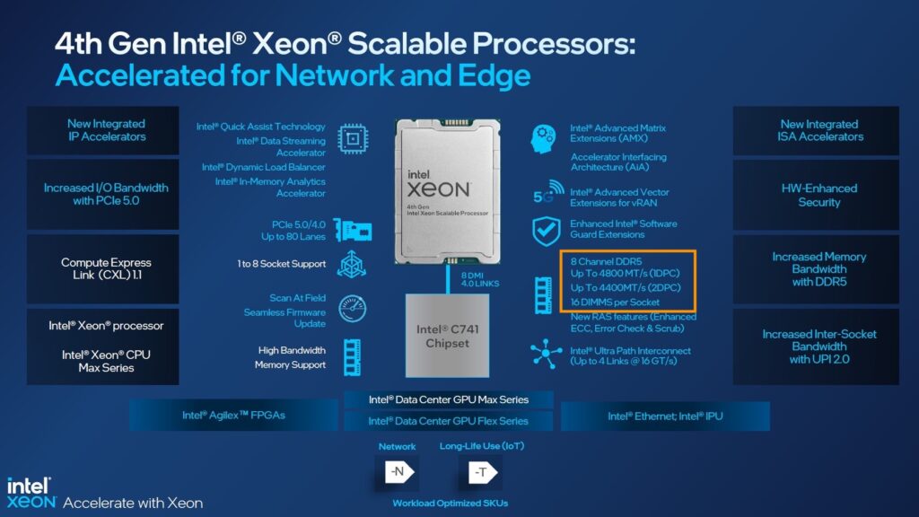
Sapphire Roads supports multiple memory speeds. The bronze and silver families support a maximum memory speed of 4000 MHz. The Gold family is all over the place, supporting a maximum of 4000, 4400, and 4800 MHz. The Platinum family supports up to 4800 MHz. However, this is in a 1 DPC configuration. 4400 MHz in a 2 DPC configuration.

The massive step up from 3200 MHz to 4800 MHz is slightly reduced when loading the server with more than eight DIMMs per CPU. When comparing theoretical bandwidth speeds, 1 DPC and 2 DPC, bandwidth performance looks as follows:

DDR4 3200 MHZ provides a theoretical bandwidth of 25.6 GB/s. DDR5 4800 MHz provides a theoretical bandwidth of 38.2 GB/s, while 4400 MHz DDR5 memory provides a theoretical bandwidth of 35.2 GB/s.

Xeon Architecture1 DPCGB/s8 Ch+%2 DPCGB/s16 Ch+%
3rd Gen Xeon3200 MHz23.4204.8 GB/s3200 MHz25.6409.6 GB/s
4th Gen Xeon4800 MHz38.4307.2 GB/s50%4400 MHz35.2563.2 GB/s37.5%

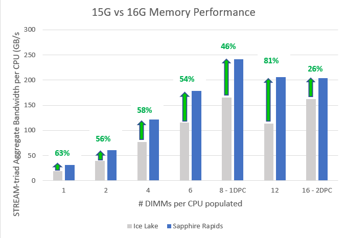
Dell published a report of performance study measuring memory bandwidth using the STREAM Triad benchmark. The study compared the performance of the 3rd and 4th generation Xeons and shows “real” bandwidth numbers. Sapphire Rapids improves memory bandwidth by 46% in a 1 DPC configuration, “but only” 26% in a 2 DPC configuration. Although STREAM is a synthetic benchmark, it does give us a better idea of what bandwidth to expect in real life.

I hope this information helps to guide you when configuring the memory configuration of your next vSphere ESXi host platform. Selecting the right DIMM capacity can quickly get 20% better memory performance.

Filed Under: CPU, Uncategorized

vSphere 8 CPU Topology Device Assignment

October 25, 2022 by frankdenneman

There seems to be some misunderstanding about the new vSphere 8 CPU Topology Device Assignment feature, and I hope this article will help you understand (when to use) this feature. This feature defines the mapping of the virtual PCIe device to the vNUMA topology. The main purpose is to optimize guest OS and application optimization. This setting does not impact NUMA affinity and scheduling of vCPU and memory locality at the physical resource layer. This is based on the VM placement policy (best effort). Let’s explore the settings and their effect on the virtual machine. Let’s go over the basics first. The feature is located in the VM Options menu of the virtual machine. 

Click on CPU Topology 

By default, the Cores per Socket and NUMA Nodes settings are “assigned at power on” and this prevents you from assigning any PCI device to any NUMA node. To be able to assign PCI devices to NUMA nodes, you need to change the Cores per Socket setting. Immediately, a warning indicates that you need to know what you are doing, as incorrectly configuring the Cores per Socket can lead to performance degradation. Typically we recommend aligning the cores per socket to the physical layout of the server. In my case, my ESXi host system is a dual-socket server, and each CPU package contains 20 cores. By default, the NUMA scheduler maps vCPU to cores for NUMA client sizing; thus, this VM configuration cannot fit inside a single physical NUMA node. The NUMA scheduler will distribute the vCPUs across two NUMA clients equally; thus, 12 vCPUs will be placed per NUMA node (socket). As a result, the Cores per Socket configuration should be 12 Cores per Socket, which will inform ESXi to create two virtual sockets for that particular VM. For completeness’ sake, I specified two NUMA nodes as well. This setting is a PER-VM setting, it is not NUMA Nodes per Socket. You can easily leave this to the default setting, as ESXi will create a vNUMA topology based on the Cores per Socket settings. Unless you want to create some funky topology that your application absolutely requires. My recommendation, keep this one set to default as much as possible unless your application developer begs you otherwise.

This allows us to configure the PCIe devices. As you might have noticed, I’ve added a PCIe device. This device is an NVIDIA A30 GPU in Dynamic Direct Path I/O (Passthrough) mode.  But before we dive into the details of this device, let’s look at the virtual machine’s configuration from within the guest OS. I’ve installed Ubuntu 22.04 LTS and used the command lstopo. (install using: sudo apt install hwloc)

You see the two NUMA nodes, with each twelve vCPUs (Cores) and a separate PCI structure. This is the way a virtual motherboard is structured. Compare this to a physical machine, and you notice that each PCI device is attached to the PCI controller that is located within the NUMA node.

And that is exactly what we can do with the device assignment feature in vSphere 8. We can provide more insights to the guest OS and the applications if they need this information. Typically, this optimization is not necessary, but for some specific network load-balancing algorithms or machine learning use cases, you want the application to understand the NUMA PCI locality of the PCIe devices. 
In the case of the A30, we need to understand its PCIe-NUMA locality. The easiest way to do this is to log on to the ESXi server through an SSH session and search for the device via the esxcli hardware pci list command. As I’m searching for an NVIDIA device, I can restrict the output of this command by using the following command “esxcli hardware pci list | grep “NVIDIA -A 32 -B 6”. This instructs the grep command to output 32 lines (A)after and 6 lines (B)before the NVIDIA line. The output shows us that the A30 card is managed by the PCI controller located in NUMA node 1 (Third line from the bottom).

We can now adjust the device assignment accordingly and assign it to NUMA node 1. Please note the feature allows you to also assign it to NUMA node 0. You are on your own here. You can do silly things. But just because you can, doesn’t mean you should. Please understand that most PCIe slots on a server motherboard are directly connected to the CPU socket, and thus a direct physical connection exists between the NIC or the GPU and the CPU. You cannot logically change this within the ESXi schedulers. The only thing you can do is to map the virtual world as close to the physical world as possible to keep everything as clear and transparent as possible. I mapped PCI device 0 (the A30) to NUMA node 1.

Running lstopo in the virtual machine provided me this result:

Now the GPU is a part of NUMA node 1. How we can confirm that is true is by taking the PCI device at address 04:00:00 given in the small green box that is inside Package 1 and seeing that is the same address as that given in the “esxcli hardware pci list” for the GPU – that is seen at the line titled “Device Layer Bus Address”  in that esxcli output. Because the virtual GPU device is now a part of NUMA node 1 the guest OS memory optimization can allocate memory within NUMA node 1 to store the dataset there so that it is as close to the device as possible. The NUMA scheduler and the CPU and memory scheduler within the ESXi layer attempt to follow these instructions to the best of their ability. If you want to be absolutely sure, you can assign NUMA affinity and CPU affinity at the lowest layers, but we recommend starting at this layer and testing this first before impacting the lowest scheduling algorithms.

Filed Under: AI & ML, CPU, NUMA

Machine Learning Workload and GPGPU NUMA Node Locality

January 30, 2020 by frankdenneman

In the previous article “PCIe Device NUMA Node Locality” I covered the physical connection between the processor and the PCIe device briefly touched upon machine learning workloads with regards to PCIe NUMA locality. This article zooms in on why it is important to consider PCIe NUMA locality.

General-Purpose Computing on Graphics Processing Units

New compute-intensive workloads take advantage of the new programming model called general-purpose computing on GPU (GPGPU). With GPGPU, the many cores integrated on modern GPUs are used to offload a vast number of (parallel) compute threads from the CPU. By adding another computational device with different characteristics, a heterogeneous compute architecture is born. GPUs are optimized for streaming sequential (or easily predictable) access patterns, while CPUs are designed for general access patterns and concurrency of threads. Combined, they form a GPGPU pipeline, that is exceptionally well-suited to analyze data. The vSphere platform is well-suited to create GPGPU pipelines and optimizations are provided to VMs, such as DirectPath I/O Access (also known as Passthrough). Passthrough allows the application to interface with the accelerator device directly; however, data must be transferred from disk/network through the system (RAM) to the GPU. And controlling the data transfer is of interest to the overall performance of the platform for both GPGPU workload and non-GPGPU workload.

A very popular GPGPU workload is Machine Learning (ML). Many ML workloads process gigabytes of data, sometimes even terabytes, this data flows from the storage device up to the PCIe device. Finetuning the configuration and placement of the virtual machine running the ML workload can benefit the data-scientist and other consumers of the platform. Not every ML workload is latency-sensitive, but most data scientists prefer to get the training done as quickly as possible. This allows them to perform more training iterations to fine-tune the model (also known as the neural network). Due to the movement of data through the system, a ML workload can quickly become the noisiest neighbor you ever saw in your system. But with the right guard-rails in place, data-scientists take advantage of running their workload on a consistent performing platform, while the rest of the organization can consume resources from this platform as well.

Machine Learning Concepts

Oversimplified ML is “using data to answer questions.” With traditional programming models, you create “rules” by using the programming language and apply these rules to the input to get output (results) (output). With ML training, you provide input and the output to train the program to create rules. This creates a predictive model that can be used to analyze previously unseen data to provide accurate answers. The key component of the entire ML process is data. This data is stored on a storage device and fetched to be used as input for the model to be trained on, or to use the trained model to provide results. Training a machine learning model is primarily done by a neural network of nodes that are executed by thousands of cores on GPUs. The nature of the cores (SIMT – Single Instruction, Multiple Data) allows for extremely fast parallel processing, ideal for this sort of workload, hence you want to use GPUs for this task and not the serial-workload optimized CPUs. The heavy lifting of the compute part is done by the GPU, but the challenge is getting the data to the costly GPU cores as fast and consistent as possible. If you do not keep the GPU cores fed with all the data it needs, then a large part of the GPU cores sit idle until new data shows up. And this is the challenge to overcome, handling large quantities of training data that flows from storage, through the host memory, into the VM memory before flowing into the memory of the GPU. High-speed storage systems with fast caching and fast paths between the storage, CPU, server memory and PCIe device are necessary.

Anatomy of an ML Training Workload

The collection of training examples is called a dataset, and the golden rule is, the more data you can use during the training, the better the predictive model becomes. That means that the data scientist will unleash copious amounts of data on the system, data so large that it cannot fit inside the memory device of the GPU. Perhaps not even the memory assigned to the virtual machine, as a result, the data is stored on disk and is retrieved in batches. 

The data scientist typically finetunes the size of the batch set, finetuning a batch set size is considered an art form in the world of ML. You, the virtual admin, slowly graduating into an ML infrastructure engineer (managing and help to design the ML platform), can help inform the data scientist by sizing the virtual machine correctly. Look at CPU consumption and determine the correct number of vCPUs necessary to push the workload. Once the GPU receives a batch, the workload is contained within the GPU. Rightsizing the VM can help to improve performance further as the VM might fit a single NUMA node.

To understand the dataflow of an ML workload through the system, let’s get familiar with some neural network terminology. Most of the ML workload use the Compute Unified Device Architecture (CUDA) for GPU programming, and when using a batch of the training data, the CUDA program takes the following steps:

1: Allocate space on the GPU device memory

2: Copy (batch set) input data to the device (aka Host to Device (HtoD))

3: Run the algorithm on the GPU cores

4: Copy output (results) back to host memory (aka Device to Host (DtoH))

During training, the program processes all the training examples in the dataset. This cycle is called an epoch. As mentioned before, a data scientist can decide to split up the entire dataset into smaller batch sets. The number of training examples used is called a batch size. An iteration is the number of passes the program needs to use to go through the entire dataset to complete a single epoch. For example, a dataset contains 100.000 samples, and each batch size contains 1000 training examples, then it takes 100 iterations to complete a single epoch. Each iteration uses the previously described CUDA loop. To get a better result, multiple epochs are pushed to get a better convergence of the training model. Within each epoch, the neural network self-tweaks its own parameters (called weights and is done for each node) in the neural network, this finetuning provides a more accurate prediction result when it’s used during the inference operation. The interesting part is that the data scientist can also make some adjustments to the (hyper)parameters of the ML model. Simply put, a hyperparameter is a parameter whose value is set before the training process begins. Such as the number of weights or the batch size set. To verify if this tuning was helpful, a new sequence of epochs is kicked off. A great series of videos about neural networks can be found here.

Josh Simons and Justin Murray gave a 4-hour workshop on ML workload on vSphere at VMworld last year. In this workshop, they stated that the typical values they saw were gigabytes of data (D), 10 to 100s of epochs (E), and 10 or more tuning cycles (T), which can be substantially more (in the 1000s) when researching new models. You can imagine that such data volumes can become a challenge in a shared system such as the hypervisor. Let’s take a look at why isolation can benefit both ML workload and the other resident workload on the system.

CPU Scheduler and NUMA optimizations

When the data is fetched from the storage device it is stored in memory. The compute schedulers of the VMkernel are optimized to store the memory as close to the CPUs as possible. Let’s use the most popular server configuration in today’s data center, the dual-socket system. Each socket contains a processor and within the processor, memory controllers exist. Memory modules (DIMMs) attached to these memory controllers are considered local memory capacity. Both processors are connected to each other to allow each processor to access the memory connected to the other processor. Due to the difference in latency and bandwidth, this is considered to be non-uniform memory access (NUMA). For more information about NUMA, check out this series.

Let use the example of a 4 vCPU VM with 32 GB, running on a host with 512GB memory with 2 processors containing 10 cores each. The dataset used is 160GB of data and it cannot be stored in the VM memory and in the GPU device memory, thus the data scientist sets the batch size to 16GB. The program fetches 16GB of training data from the datastore and the NUMA scheduler ensures the data is stored within the local memory of the processor the four vCPU run on. In this case, the vCPUs of the VM are scheduled on the cores of CPU 1 (NUMA node 1) and thus the NUMA scheduler requests the VMkernel memory scheduler to store it in the memory pages belonging to the memory address space managed by the memory controllers of CPU 1.

The VM is configured with a passthrough GPU and the training data is pushed to the GPU. The problem is that the GPU is manually selected by the admin and no direct relation is visible in the UI or command-line, it just shows the type name and a PCI address. GPUs are PCIe devices and they are hardwired and controlled by a CPU.

The admin selected the first GPU in the list and now the dataset is pushed directly from the VM memory to the GPU Device memory to be used by the cores of the GPU. Data now flows through the interconnect to the PCIe controller of CPU 0 and to the GPU device. Each dataset that is retrieved from storage, is stored in NUMA node 1 and then moved through the interconnect to the device, this is done for each iteration, for each epoch and this can be done 1000’s of time.

The problem is that the interconnect is used by the entire system. When the CPU needs to rebalance, it can reschedule the vCPU on cores belonging to a different CPU if this improves the overall resource availability for the active virtual machines. Memory can be transferred over to the new NUMA home node of that recently migrated virtual machine, or memory is just accessed across the interconnect. Same with Wide-VMs, VMs that span multiple NUMA nodes, it can happen that these Wide-VMs access a lot of “remote” memory. Also do not forget the data being handled by other PCIe devices. All network traffic has to flow from the NIC to a particular VM, for optimized performance, the kernel prefers to store that data in memory that is local to the vCPUs of that VM. The same goes for data coming from external storage devices, if the HBA or NIC is “hanging” off the other CPU, data has to flow through the interconnect. The interconnect is a highway shared by a lot of components and workloads. These operations can impact the performance of the ML workload but the opposite is also true, pushing 1000 epochs of gigabytes of data to a GPU ensures other workloads will notice the presence of that workload, even if it has a small CPU and memory footprint. Remember, ML is “using data to answer questions.”

PTNumaTopology PowerCLI Module

To make sense of it all, I created a simple PowerCLI module with two functions that show the VMs that have a passthrough device configured. The output shows the VM name and the PCI address of the device so that you can relate that to what you see in the UI. The next column shows the NUMA node to which the PCIe device is connected. The next column indicates whether the advanced setting numa.affinity is set for that particular VM and its value. The last column shows the power state of the VM. To set the NUMA affinity, the VM has to be powered off.

To run the script, import the module (available at GitHub) and execute the Get-PTNumaTopology command. Specify the FQDN of the ESXi host. For example: Get-PTNumaTopology -esxhost sc2esx27.vslab.local. As the script needs to execute a command on the ESXi host locally an SSH session is initiated. This results in a prompt for a (root) username and password in a separate login screen. (The Github page has a thorough walk-through of all the steps involved and a list of requirements.)

NUMA Affinity Advanced Setting

In most situations, it is not recommended to set any affinity setting as it simply restricts the scheduler to generate an optimal balance between resource providers (CPUs) and consumers (vCPUs). At the host level and cluster level. However since the VM is configured with a passthrough (PT) GPU, it cannot move to another host and chances are a lot of data will flow to this device. Another assumption is that the host contains a small number of GPUs and thus a small number of VMs are active. If no other restrictions are configured, the CPU and NUMA scheduler can try to work “around” the affined VM and attempt to optimize the placement and resource consumptions of the other active VMs. Hopefully, the isolation of these particular passthrough-enabled VMs are reducing overall system load and thus evening out the possible enforced restrictions. Testing this first before using it on the production workload is always recommended! For more information about the NUMA affinity setting, please consult the VMware Docs for your specific vSphere version, linked is the VMware Docs page for vSphere 6.7.

Why set numa.affinity and not use CPU pinning? First of all, CPU pinning is something that should not be done ever. And even when you think you have a valid use case, chances are that CPU pinning will still reduce performance significantly. This topic is rearing its ugly head again and I will soon post another article why CPU pinning is just a bad idea. NUMA affinity creates a rule for the CPU scheduler to find a CPU core or HT within the boundaries of the CPU itself. In the example of the 4 vCPU running on the 10 core CPU. Let’s say hyperthreading is enabled, it allows the CPU scheduler to schedule one of these four CPUs on the 20 available logical processors. If the system is not over-utilized, it can use a complete core for a vCPU, it can find the optimal placement for that workload and for the others using the same CPU. With pinning you restrict the vCPUs to only run on that particular logical processor. If chosen incorrectly you might have just selected HTs only.

If you decide to set a NUMA affinity on a particular VM, the Get-PTNumaTopology function can help you to set it correctly. As a failsafe, the script proceeds to ask if you would like to set the NUMA node affinity of a powered off VM. Answer “N” to end the script and return to the command-line. If you answer “Y” for yes, it will then ask you to provide the name of the VM. Please note that this setting can only be applied on a powered-off VM. Setting an advanced setting means that the system is writing to this to the VMX file and the VMX file is in a locked state during the power-on state of a VM. The next step is to provide the NUMA Node you want the vCPUs to set the affinity for. Use the same number listed in the PCI NUMA Node column behind the attached passthrough device.

Once the advanced setting is configurated it shows the configured value. To verify whether the setting matches the NUMA node of the passthrough device, run the command Get-PTNumaTopology again. As it has closed the SSH connection after the last run, you are required to log in again with the root user account to retrieve the current settings.

Setting the NUMA node advanced option for a VM is something that should be done for specific reasons, do not use the script for all your virtual machines. The NUMA affinity setting applies to the placement of vCPU only. The NUMA scheduler provides recommendations to the memory scheduler, but it is up to the memory scheduler discretion to store the data. The kernel is optimized to keep the memory close to the vCPUs as possible, but sometimes it cannot fit that memory into that node. Either because the VM configuration exceeds the total capacity of that node, or that other active VMs are already using large amounts of memory of that node. Setting the affinity is not a 100% guarantee that all the resources are local, but in the majority of use-cases, it will. Isolating the workload within a specific NUMA node will help to provide you consistent performance and will reduce a lot of interconnect bandwidth consumption. Enjoy using the script!

Font used in PowerShell environment: JetBrains Mono – available at – https://www.jetbrains.com/lp/mono/#intro

Filed Under: AI & ML, CPU, NUMA Tagged With: GPGPU, GPU, Machine Learning, NUMA, PCIe, VMware, vSphere

Explainer on #Spectre & #Meltdown by Graham Sutherland

January 5, 2018 by frankdenneman

Sometimes you stumble across a brilliant Twitter thread, so good, that it should never be lost. Graham Sutherland (@gsuberland) helped the world in understanding the Spectre and Meltdown bugs. I’m publishing his tweet thread in text form as this is just the best explanation of the bugs I’ve seen.
Please note that VMware has released its response for Bounds-Check Bypass (CVE-2017-5753), Branch Target Injection (CVE-2017-5715) & Rogue Data Cache Load (CVE-2017-5754) – AKA Meltdown & Spectre.

https://blogs.vmware.com/security/2018/01/vmsa-2018-0002.html
Disclaimer: All text below is produced by Graham Sutherland, I’m not taking any credits for this work

Explainer on #Spectre & #Meltdown:

When a processor reaches a conditional branch in code (e.g. an 'if' clause), it tries to predict which branch will be taken before it actually knows the result. It executes that branch ahead of time – a feature called "speculative execution".

— Graham Sutherland (Polynomial^DSS) ➡️ chaos.social (@gsuberland) January 4, 2018

Explainer on #Spectre & #Meltdown:
When a processor reaches a conditional branch in code (e.g. an ‘if’ clause), it tries to predict which branch will be taken before it actually knows the result. It executes that branch ahead of time – a feature called “speculative execution”.

The idea is that if it gets the prediction right (which modern processors are quite good at) it’ll already have executed the next bit of code by the time the actually-selected branch is known. If it gets it wrong, execution unwinds back and the correct branch is executed instead.
What makes the processor so good at branch prediction is that it stores details about previous branch operations, in what’s called the Branch History Buffer (BHB). If a particular branch instruction took path A before, it’ll probably take path A again, rather than path B.
What makes this interesting is that code is executed *speculatively*, before the result of a conditional statement has completed. That conditional statement could be security-critical. Thankfully the processor is (mostly) smart enough to roll back any side-effects of execution.
There are two important exclusions to the rollback of side-effects: cache and branch prediction history. These generally aren’t rolled back because speculative execution is a performance feature, and rolling back cache and BHB contents would generally hurt performance.
There are three ways to exploit this behaviour. The Spectre paper describes the first two exploits, with the following results:
1. Kernel memory disclosure from userspace on bare metal.
2. Kernel memory disclosure of the VM host/hypervisor from kernelspace in a VM.
The first exploit works by getting the kernel to execute some carefully written attacker-specified code which contains an array bounds check followed by an array read, where the read index is controlled by an attacker. This sounds like a big ask, but it’s not thanks to JIT.
On Linux, Extended Berkley Packet Filter (eBPF) allows users to write socket filters from usermode which get JIT compiled by the kernel in order to efficiently filter packets on a socket. The details aren’t important, but it means an attacker can get the kernel to execute code.
The exploit involves writing eBPF code which compiles to the following steps:
1. Allocate two fixed-size arrays
2. Bounds-check the user-provided index
3. If ok, read from the array1 at that index
4. Compute another index from 1 bit of the result
5. Read from array2 at that index
There’s actually a step before 5, which is “bounds check the read to array2”, but we never intend to do an out-of-bounds read here, so it’s irrelevant. I omitted it because I ran out of characters.
In terms of “real” execution, this code always terminates at step 2 when the user passes an out-of-bounds index for array1. But if the processor’s branch predictor assumes that check will succeed, it’ll speculatively execute the out-of-bounds read in step 3, and continue to 5.
Here’s the clever bit. In step 4 we take the value we got from the out-of-bounds read (which we wouldn’t normally have access to) and use one bit from it to select a particular memory address (array index) to read. If b=0 it reads index 0x200; if b=1 it reads index 0x300.
This ensures that the memory at either index 0x200 or index 0x300 is now cached. The CPU then realises that the bounds check in step 2 failed, so it unwinds back to that branch. However, the data from step 5 is still cached!
We can then go in and read the data at 0x200 and 0x300 and see which is cached by measuring how quick the read is. Once we know which index was cached we can directly infer one bit of kernel memory, based on the index selection from step 4.
There are some details as to how the cache needs to be primed before this attack, but it is possible to do this whole process in a loop and dump kernel memory from unprivileged userspace.
The second attack described in the Spectre paper involves poisoning the branch prediction history to trick the processor into speculatively executing code at an attacker-specified address, leading to further cache attacks as described above.
By performing a carefully selected sequence of indirect jumps, an attacker can fill up the branch prediction history in a way that allows the attacker to select which branch will be speculatively executed when performing an indirect jump.
This can be very powerful. If I know there’s a piece of code in kernel space that exhibits similar behaviour to our eBPF example from before, and I know what the address of that code is, I can indirectly jump to that code and the CPU will speculatively execute it.
If you’ve done exploitation before, you’ll probably recognise this as being similar to a ROP gadget. We’re looking for a sequence of code in kernel space that happens to have the right sequence of instructions to leak information via cache.
Keep in mind that the execution is speculative only – the processor will later realise that I didn’t have the privilege to jump to that code and throw an exception. So the target code has to leak kernel data via cache side-channels like before.
You’ll also notice that we need to know address of the target kernel code. With KASLR this isn’t so easy. Project Zero’s writeup explains how KASLR can be defeated using branch prediction and caching as side-channels, so I won’t go into the details here.
https://googleprojectzero.blogspot.co.uk/2018/01/reading-privileged-memory-with-side.html
What makes this extra powerful is that it works across VM boundaries too. Instead of a traditional indirect jump (e.g. jmp eax), we can use the vmcall instruction to speculatively execute code within the VM host’s kernel in the same way we would our VM’s kernel.
Finally, there’s the third approach. This involves a flush+reload cache attack against kernel memory, similar to the first variant of the attack but without requiring kernel code execution – it can all be done from usermode.
The idea is that we try to read kernelspace memory using a mov instruction, then perform a secondary memory read with an address based on the value that was read. If you’re thinking the first mov will fail because we’re in usermode and can’t read kernel addresses, you’re right.
The trick is that the microarchitectural implementation of mov contains the memory page privilege level check, which itself is a branch instruction. The processor may speculatively execute that branch like any other.
So, if you can outrun the interrupt, you can speculatively execute some other instruction that loads data into cache based on the value read from kernelspace. This then becomes a cache attack like the previous tricks.
And that’s just about it.
For full details I recommend checking out the two papers, as well as the Project Zero writeup I linked above.
https://spectreattack.com/spectre.pdf
https://meltdownattack.com/meltdown.pdf
Thanks Graham for this excellent explanation!

Filed Under: CPU, VMware

Why the Recent Reported Intel HT Bug is Not in Your Data Center

June 26, 2017 by frankdenneman

Yesterday I tweeted out the warning message about the HT bug of Skylake and Kaby Lake processors posted on debian.org.
https://lists.debian.org/debian-devel/2017/06/msg00308.html
My tweet got a LOT of retweets. A lot replied with concerns about their systems. I believe most Data Centers will not suffer from this bug as it is present on Skylake and Kaby Lake processors.
What is the Bug?
According to the warning: Unfixed Skylake and Kaby Lake processors could, in some
situations, dangerously misbehave when hyper-threading is enabled.
Disable hyper-threading immediately in BIOS/UEFI to work around the problem. Read this advisory for instructions about an Intel-provided fix.
https://www.intel.com/content/www/us/en/processors/xeon/xeon-e3-1200v5-spec-update.html

Unlikely Present in Your Data Center
The reason why I believe most systems in data centers are not hit by this bug is that it solely applies to E3 Xeons from the Skylake microarchitecture. E3 CPUs are designed to operate in a single socket system, they have no QuickPath Interconnect. Therefore unable to create a symmetric multiprocessing system.
The current E5 (dual-socket) system is based on the Broadwell microarchitecture. The Skylake microarchitecture is expected to appear within the next couple of months. According to the report, they will have the fix included when the product launched. If you are running a NUC in your lab, you might want to check to see whether your system might hit that bug
http://ark.intel.com/products/codename/82879/Kaby-Lake
http://ark.intel.com/products/codename/37572/Skylake
The link will forward you to a perl script that can help detect if your
system is affected or not. Many thanks to Uwe Kleine-König for
suggesting, and writing this script.
https://lists.debian.org/debian-devel/2017/06/msg00309.html
–

Filed Under: CPU

  • Page 1
  • Page 2
  • Go to Next Page »

Copyright © 2025 · SquareOne Theme on Genesis Framework · WordPress · Log in