• Skip to primary navigation
  • Skip to main content

frankdenneman.nl

  • AI/ML
  • NUMA
  • About Me
  • Privacy Policy

Search Results for: machine learning

Machine Learning Workload and GPGPU NUMA Node Locality

January 30, 2020 by frankdenneman

In the previous article “PCIe Device NUMA Node Locality” I covered the physical connection between the processor and the PCIe device briefly touched upon machine learning workloads with regards to PCIe NUMA locality. This article zooms in on why it is important to consider PCIe NUMA locality.

General-Purpose Computing on Graphics Processing Units

New compute-intensive workloads take advantage of the new programming model called general-purpose computing on GPU (GPGPU). With GPGPU, the many cores integrated on modern GPUs are used to offload a vast number of (parallel) compute threads from the CPU. By adding another computational device with different characteristics, a heterogeneous compute architecture is born. GPUs are optimized for streaming sequential (or easily predictable) access patterns, while CPUs are designed for general access patterns and concurrency of threads. Combined, they form a GPGPU pipeline, that is exceptionally well-suited to analyze data. The vSphere platform is well-suited to create GPGPU pipelines and optimizations are provided to VMs, such as DirectPath I/O Access (also known as Passthrough). Passthrough allows the application to interface with the accelerator device directly; however, data must be transferred from disk/network through the system (RAM) to the GPU. And controlling the data transfer is of interest to the overall performance of the platform for both GPGPU workload and non-GPGPU workload.

A very popular GPGPU workload is Machine Learning (ML). Many ML workloads process gigabytes of data, sometimes even terabytes, this data flows from the storage device up to the PCIe device. Finetuning the configuration and placement of the virtual machine running the ML workload can benefit the data-scientist and other consumers of the platform. Not every ML workload is latency-sensitive, but most data scientists prefer to get the training done as quickly as possible. This allows them to perform more training iterations to fine-tune the model (also known as the neural network). Due to the movement of data through the system, a ML workload can quickly become the noisiest neighbor you ever saw in your system. But with the right guard-rails in place, data-scientists take advantage of running their workload on a consistent performing platform, while the rest of the organization can consume resources from this platform as well.

Machine Learning Concepts

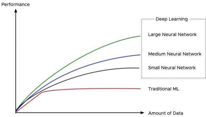
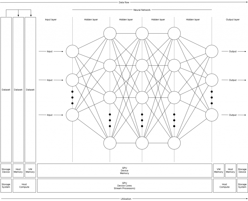
Oversimplified ML is “using data to answer questions.” With traditional programming models, you create “rules” by using the programming language and apply these rules to the input to get output (results) (output). With ML training, you provide input and the output to train the program to create rules. This creates a predictive model that can be used to analyze previously unseen data to provide accurate answers. The key component of the entire ML process is data. This data is stored on a storage device and fetched to be used as input for the model to be trained on, or to use the trained model to provide results. Training a machine learning model is primarily done by a neural network of nodes that are executed by thousands of cores on GPUs. The nature of the cores (SIMT – Single Instruction, Multiple Data) allows for extremely fast parallel processing, ideal for this sort of workload, hence you want to use GPUs for this task and not the serial-workload optimized CPUs. The heavy lifting of the compute part is done by the GPU, but the challenge is getting the data to the costly GPU cores as fast and consistent as possible. If you do not keep the GPU cores fed with all the data it needs, then a large part of the GPU cores sit idle until new data shows up. And this is the challenge to overcome, handling large quantities of training data that flows from storage, through the host memory, into the VM memory before flowing into the memory of the GPU. High-speed storage systems with fast caching and fast paths between the storage, CPU, server memory and PCIe device are necessary.

Anatomy of an ML Training Workload

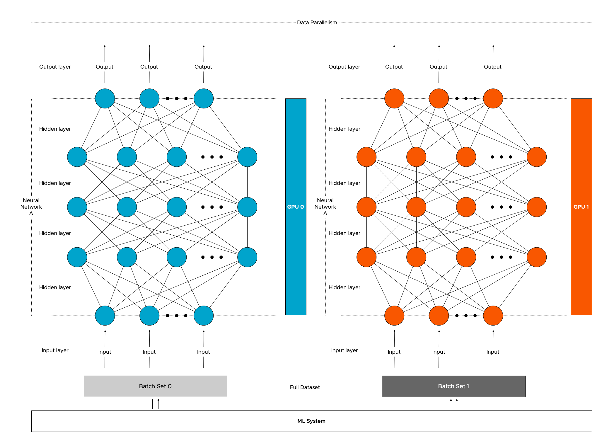
The collection of training examples is called a dataset, and the golden rule is, the more data you can use during the training, the better the predictive model becomes. That means that the data scientist will unleash copious amounts of data on the system, data so large that it cannot fit inside the memory device of the GPU. Perhaps not even the memory assigned to the virtual machine, as a result, the data is stored on disk and is retrieved in batches. 

The data scientist typically finetunes the size of the batch set, finetuning a batch set size is considered an art form in the world of ML. You, the virtual admin, slowly graduating into an ML infrastructure engineer (managing and help to design the ML platform), can help inform the data scientist by sizing the virtual machine correctly. Look at CPU consumption and determine the correct number of vCPUs necessary to push the workload. Once the GPU receives a batch, the workload is contained within the GPU. Rightsizing the VM can help to improve performance further as the VM might fit a single NUMA node.

To understand the dataflow of an ML workload through the system, let’s get familiar with some neural network terminology. Most of the ML workload use the Compute Unified Device Architecture (CUDA) for GPU programming, and when using a batch of the training data, the CUDA program takes the following steps:

1: Allocate space on the GPU device memory

2: Copy (batch set) input data to the device (aka Host to Device (HtoD))

3: Run the algorithm on the GPU cores

4: Copy output (results) back to host memory (aka Device to Host (DtoH))

During training, the program processes all the training examples in the dataset. This cycle is called an epoch. As mentioned before, a data scientist can decide to split up the entire dataset into smaller batch sets. The number of training examples used is called a batch size. An iteration is the number of passes the program needs to use to go through the entire dataset to complete a single epoch. For example, a dataset contains 100.000 samples, and each batch size contains 1000 training examples, then it takes 100 iterations to complete a single epoch. Each iteration uses the previously described CUDA loop. To get a better result, multiple epochs are pushed to get a better convergence of the training model. Within each epoch, the neural network self-tweaks its own parameters (called weights and is done for each node) in the neural network, this finetuning provides a more accurate prediction result when it’s used during the inference operation. The interesting part is that the data scientist can also make some adjustments to the (hyper)parameters of the ML model. Simply put, a hyperparameter is a parameter whose value is set before the training process begins. Such as the number of weights or the batch size set. To verify if this tuning was helpful, a new sequence of epochs is kicked off. A great series of videos about neural networks can be found here.

Josh Simons and Justin Murray gave a 4-hour workshop on ML workload on vSphere at VMworld last year. In this workshop, they stated that the typical values they saw were gigabytes of data (D), 10 to 100s of epochs (E), and 10 or more tuning cycles (T), which can be substantially more (in the 1000s) when researching new models. You can imagine that such data volumes can become a challenge in a shared system such as the hypervisor. Let’s take a look at why isolation can benefit both ML workload and the other resident workload on the system.

CPU Scheduler and NUMA optimizations

When the data is fetched from the storage device it is stored in memory. The compute schedulers of the VMkernel are optimized to store the memory as close to the CPUs as possible. Let’s use the most popular server configuration in today’s data center, the dual-socket system. Each socket contains a processor and within the processor, memory controllers exist. Memory modules (DIMMs) attached to these memory controllers are considered local memory capacity. Both processors are connected to each other to allow each processor to access the memory connected to the other processor. Due to the difference in latency and bandwidth, this is considered to be non-uniform memory access (NUMA). For more information about NUMA, check out this series.

Let use the example of a 4 vCPU VM with 32 GB, running on a host with 512GB memory with 2 processors containing 10 cores each. The dataset used is 160GB of data and it cannot be stored in the VM memory and in the GPU device memory, thus the data scientist sets the batch size to 16GB. The program fetches 16GB of training data from the datastore and the NUMA scheduler ensures the data is stored within the local memory of the processor the four vCPU run on. In this case, the vCPUs of the VM are scheduled on the cores of CPU 1 (NUMA node 1) and thus the NUMA scheduler requests the VMkernel memory scheduler to store it in the memory pages belonging to the memory address space managed by the memory controllers of CPU 1.

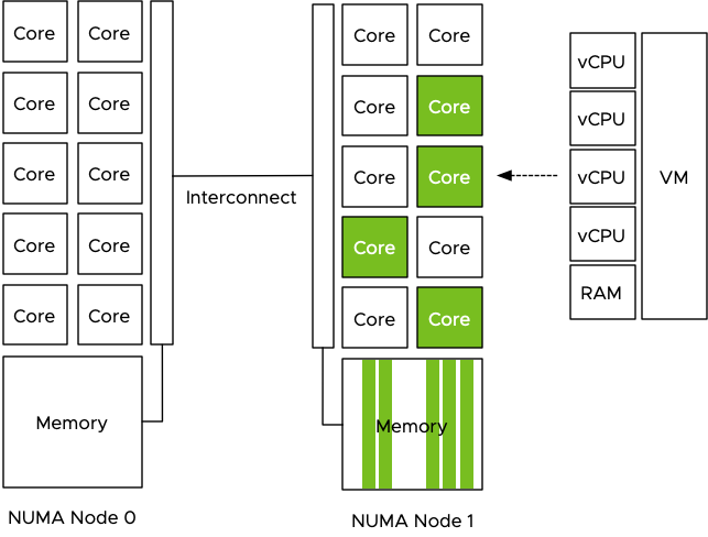
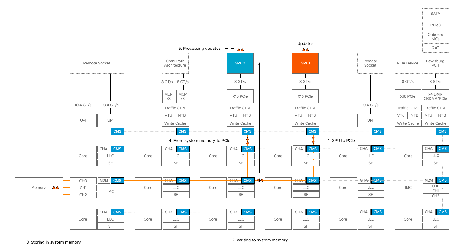
The VM is configured with a passthrough GPU and the training data is pushed to the GPU. The problem is that the GPU is manually selected by the admin and no direct relation is visible in the UI or command-line, it just shows the type name and a PCI address. GPUs are PCIe devices and they are hardwired and controlled by a CPU.

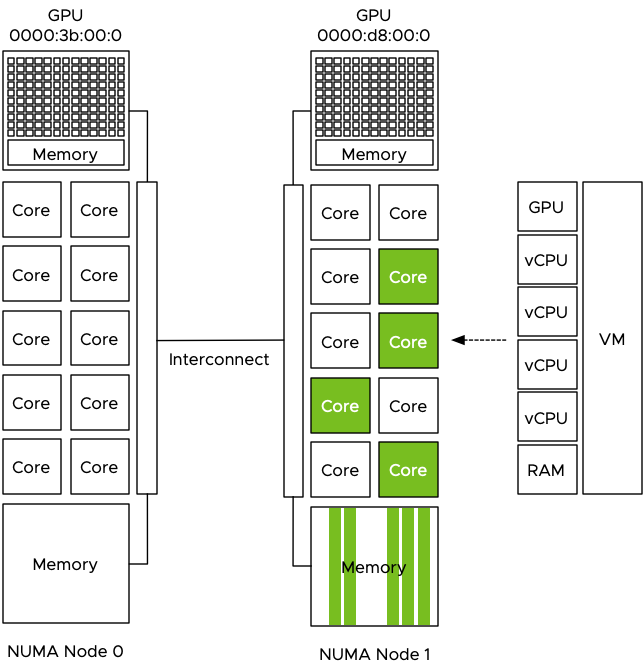
The admin selected the first GPU in the list and now the dataset is pushed directly from the VM memory to the GPU Device memory to be used by the cores of the GPU. Data now flows through the interconnect to the PCIe controller of CPU 0 and to the GPU device. Each dataset that is retrieved from storage, is stored in NUMA node 1 and then moved through the interconnect to the device, this is done for each iteration, for each epoch and this can be done 1000’s of time.

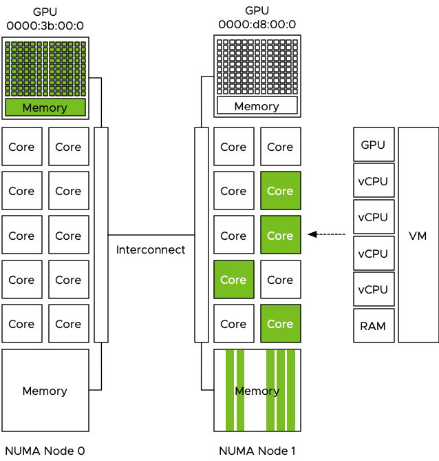
The problem is that the interconnect is used by the entire system. When the CPU needs to rebalance, it can reschedule the vCPU on cores belonging to a different CPU if this improves the overall resource availability for the active virtual machines. Memory can be transferred over to the new NUMA home node of that recently migrated virtual machine, or memory is just accessed across the interconnect. Same with Wide-VMs, VMs that span multiple NUMA nodes, it can happen that these Wide-VMs access a lot of “remote” memory. Also do not forget the data being handled by other PCIe devices. All network traffic has to flow from the NIC to a particular VM, for optimized performance, the kernel prefers to store that data in memory that is local to the vCPUs of that VM. The same goes for data coming from external storage devices, if the HBA or NIC is “hanging” off the other CPU, data has to flow through the interconnect. The interconnect is a highway shared by a lot of components and workloads. These operations can impact the performance of the ML workload but the opposite is also true, pushing 1000 epochs of gigabytes of data to a GPU ensures other workloads will notice the presence of that workload, even if it has a small CPU and memory footprint. Remember, ML is “using data to answer questions.”

PTNumaTopology PowerCLI Module

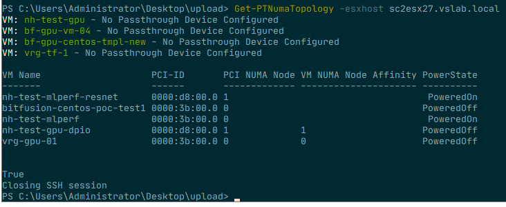
To make sense of it all, I created a simple PowerCLI module with two functions that show the VMs that have a passthrough device configured. The output shows the VM name and the PCI address of the device so that you can relate that to what you see in the UI. The next column shows the NUMA node to which the PCIe device is connected. The next column indicates whether the advanced setting numa.affinity is set for that particular VM and its value. The last column shows the power state of the VM. To set the NUMA affinity, the VM has to be powered off.

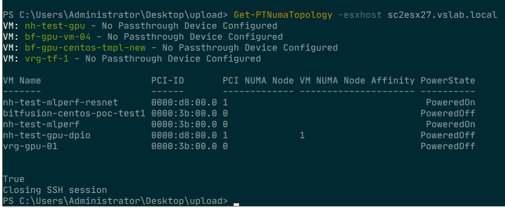
To run the script, import the module (available at GitHub) and execute the Get-PTNumaTopology command. Specify the FQDN of the ESXi host. For example: Get-PTNumaTopology -esxhost sc2esx27.vslab.local. As the script needs to execute a command on the ESXi host locally an SSH session is initiated. This results in a prompt for a (root) username and password in a separate login screen. (The Github page has a thorough walk-through of all the steps involved and a list of requirements.)

NUMA Affinity Advanced Setting

In most situations, it is not recommended to set any affinity setting as it simply restricts the scheduler to generate an optimal balance between resource providers (CPUs) and consumers (vCPUs). At the host level and cluster level. However since the VM is configured with a passthrough (PT) GPU, it cannot move to another host and chances are a lot of data will flow to this device. Another assumption is that the host contains a small number of GPUs and thus a small number of VMs are active. If no other restrictions are configured, the CPU and NUMA scheduler can try to work “around” the affined VM and attempt to optimize the placement and resource consumptions of the other active VMs. Hopefully, the isolation of these particular passthrough-enabled VMs are reducing overall system load and thus evening out the possible enforced restrictions. Testing this first before using it on the production workload is always recommended! For more information about the NUMA affinity setting, please consult the VMware Docs for your specific vSphere version, linked is the VMware Docs page for vSphere 6.7.

Why set numa.affinity and not use CPU pinning? First of all, CPU pinning is something that should not be done ever. And even when you think you have a valid use case, chances are that CPU pinning will still reduce performance significantly. This topic is rearing its ugly head again and I will soon post another article why CPU pinning is just a bad idea. NUMA affinity creates a rule for the CPU scheduler to find a CPU core or HT within the boundaries of the CPU itself. In the example of the 4 vCPU running on the 10 core CPU. Let’s say hyperthreading is enabled, it allows the CPU scheduler to schedule one of these four CPUs on the 20 available logical processors. If the system is not over-utilized, it can use a complete core for a vCPU, it can find the optimal placement for that workload and for the others using the same CPU. With pinning you restrict the vCPUs to only run on that particular logical processor. If chosen incorrectly you might have just selected HTs only.

If you decide to set a NUMA affinity on a particular VM, the Get-PTNumaTopology function can help you to set it correctly. As a failsafe, the script proceeds to ask if you would like to set the NUMA node affinity of a powered off VM. Answer “N” to end the script and return to the command-line. If you answer “Y” for yes, it will then ask you to provide the name of the VM. Please note that this setting can only be applied on a powered-off VM. Setting an advanced setting means that the system is writing to this to the VMX file and the VMX file is in a locked state during the power-on state of a VM. The next step is to provide the NUMA Node you want the vCPUs to set the affinity for. Use the same number listed in the PCI NUMA Node column behind the attached passthrough device.

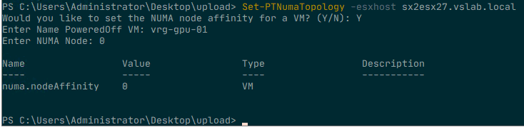
Once the advanced setting is configurated it shows the configured value. To verify whether the setting matches the NUMA node of the passthrough device, run the command Get-PTNumaTopology again. As it has closed the SSH connection after the last run, you are required to log in again with the root user account to retrieve the current settings.

Setting the NUMA node advanced option for a VM is something that should be done for specific reasons, do not use the script for all your virtual machines. The NUMA affinity setting applies to the placement of vCPU only. The NUMA scheduler provides recommendations to the memory scheduler, but it is up to the memory scheduler discretion to store the data. The kernel is optimized to keep the memory close to the vCPUs as possible, but sometimes it cannot fit that memory into that node. Either because the VM configuration exceeds the total capacity of that node, or that other active VMs are already using large amounts of memory of that node. Setting the affinity is not a 100% guarantee that all the resources are local, but in the majority of use-cases, it will. Isolating the workload within a specific NUMA node will help to provide you consistent performance and will reduce a lot of interconnect bandwidth consumption. Enjoy using the script!

Font used in PowerShell environment: JetBrains Mono – available at – https://www.jetbrains.com/lp/mono/#intro

Filed Under: AI & ML, CPU, NUMA Tagged With: GPGPU, GPU, Machine Learning, NUMA, PCIe, VMware, vSphere

Deep Learning Technology Stack Overview for the vAdmin – Part 1

March 12, 2020 by frankdenneman

Introduction

We are amid the AI “gold rush.” More organizations are looking to incorporate any form of machine learning (ML) or deep learning in their services to enhance customer experience, drive efficiencies in their processes or improve quality of life (healthcare, transportation, smart cities).  

Train Where Data is Generated

One of the key elements that drive on-premise ML focused infrastructure growth is the reality of data gravity. Mentioned in the article “Multi-GPU and Distributed Deep Learning,” deep learning (DL) gets better with data. Consequently, data sets used for ML and DL training purposes are growing at a tremendous rate. These vast data sets need to be processed. Data transit, hosting, and the necessary compute cycles impact the overall OPEX budget. Additionally, data protection regulations such as data residency, data sovereignty, and data locality impact where data can be stored outside the place it is created. As a result, a lot of forward-leaning organizations are repatriating their AI platforms to run ML and DL workloads close to the systems that generate the data. 

And what better platform to run ML and DL workloads than vSphere? Machine learning comes with its own set of lingo, and different personas interacting with the machine learning stack. To be able to have a meaningful conversation with data scientists and ML engineers, you need to have a basic understanding of how each component interacts with each other. You don’t have to learn the ins and out of the different neural networks, but having an idea of what a particular component does help you understand how it might impact your service levels and your selection of components of the vSphere platform used for ML workloads.

To give an example, OpenCL and Vulkan are frameworks that allow for the execution of code on GPU (General Purpose GPU). Using this framework allows you to theoretically expose any GPUs to a machine learning framework such as Tensorflow or Pytorch. As it’s open-source, you can use it on all kinds of GPUs from different vendors. However, all popular actively-developed frameworks do not support OpenCL or Vulkan and only use the NVIDIA CUDA API framework, thus impacting your hardware selection for the vSphere host design. I created an overview of the different layers of the deep learning technology stack, attempting to make sense of the relationships between the components of each different layer. 

Deep Learning Technology Stack

Let’s use a bottom-up approach for reviewing the deep learning technology stack.

vSphere Constructs and Accelerators

Hardware over the last 20 years looked uniform, other than the vendor and some minor vendor-specific functionality; the devices appeared relatively similar to a guest OS. Most code can run on an AMD as well as an Intel without changing. Hardware competed on scale and speed, not on different ways how it can interact with software. Today’s acceleration devices are very diverse and expose their explicit architecture to the application. The hardware specifics determine the code and algorithm used in the application. And therefore, we need to expose these devices to the application in its most raw and unique form. As a result, the overview primarily covers acceleration devices such as GPUs and FPGAs. 

However, recently Rice University released a new research paper called: “SLIDE: In Defense of Smart Algorithms over Hardware Acceleration for Large-Scale Deep Learning Systems“. They are demonstrating that by using a fundamentally different approach, it is possible to accelerate deep learning without using hardware accelerators like GPUs.

Our evaluations on industry-scale recommendation datasets, with large fully connected architectures, show that training with SLIDE on a 44 core CPU is more than 3.5 times (1-hour vs. 3.5 hours) faster than the same network trained using TF on Tesla V100 at any given accuracy level. On the same CPU hardware, SLIDE is over 10x faster than TF

I assume the authors meant a dual-socket system with two 22-cores Xeon CPUs, but an exciting development that certainly needs to be closely followed. For now, let’s concentrate on the components used by the majority of the deep-learning community.

vSphere can expose the accelerator devices via two constructs right now, DirectPath I/O (Passthrough) and NVIDIA vGPU. In 2020 two additional constructs will be available; Dynamic DirectPath I/O (information will follow soon) and Bitfusion. Bitfusion pools and shares accelerators across VMs inside the cluster. It provides virtual remote attached GPUs that can be shared between VMs fully or fractionally. Bitfusion can even assign multiple GPUs to a single VM to support any form of distributed deep learning strategy.

DirectPath I/O

DirectPath I/O, often called Passthrough, provides similar functionality as bare-metal GPU. DirectPath I/O is used for maximum hardware device performance inside the VM and to use native vendor driver and app stack support in the guest OS and the application. Perfect for running specialized software libraries provided by the CUDA stack, which is covered in a later paragraph. DirectPath I/O allows for maximum performance because the I/O mapped from the application and guest OS directly to the hardware device; the VMkernel (Hypervisor) is not involved. 

A complete device is assigned to a single VM and cannot be shared with other active VMs. This prohibits fractional use of the device (i.e., assigning half of the device resources to a VM). DirectPath I/O allows assigning multiple GPUs to a VM.

When a DirectPath I/O device is assigned to a virtual machine, it uses the physical location of the device for the assignment, i.e., Host:Bus: Device-Physical-Function. (The article “Machine Learning Workload and GPGPU NUMA Node Locality” describes locality assignment in detail). Due to this, DirectPath I/O is not compatible with certain core virtualization features, such as vMotion (and thus DRS).

Design Impact

Currently, vSphere does not support the AMD Radeon Server Accelerators for Deep learning (Radeon Instinct). vSphere supports only NVIDIA GPUs at the moment. From vSphere 6.7 update 1, FPGAs can also be directly exposed to the guest OS by using DirectPath I/O. At the time of writing this article, vSphere 6.7 update 1 supports the Intel Arria 10 GX FPGA. More details on the vSphere blog.

NVIDIA vGPU

NVIDIA virtual GPU (vGPU) provides advanced GPU virtualization functionality that enables the sharing of GPU devices across VMs. An NVIDIA GPU can be logically partitioned (fractional GPU) to multiple virtual GPUs. A VM can use multiple vGPUs that are located in the same host. Both the hypervisor and the VM need to run NVIDIA software to provide fractional, full, and multiple vGPU functionalities.

Bitfusion

In 2019, VMware acquired Bitfusion, and I’m looking forward to having this functionality available to our customers. Bitfusion FlexDirect software allows for pooling GPU resources and providing a dynamic remote attach service. That means that workload can run on vSphere hosts that do not have GPU hardware installed. The beauty of this solution is that it does not require any changes to the application. It uses native CUDA (see acceleration libraries paragraph) to intercept the application calls, the FlexDirect software sends it to the FlexDirect server across the network. The Flexdirect server has a DirectPath I/O connection to all the GPUs in that host and manages the placement and scheduling of the workloads.

This model corresponds heavily to the early days of virtualization. We used to have 1000’s x86 servers in the data center, each having an average utilization of less than 10% while costing a lot of money. We consolidated compute resources and managed the workload in such a manner than peak utilization did not overlap. With the rise of general-purpose computing on GPU, we see the same patterns. The GPUs are not cheap, sometimes the cost of a GPU server is an order of magnitude more expensive than a “traditional” server. However, when we look at the utilization, we see an average usage of 5 to 20%.

Deep Learning Development Cycle
With deep-learning, you cannot just pump some data into a deep-learning model and expect a result. The data scientist has to gather training data, asses the data quality. The next step is to choose an algorithm and a framework. Often the data is not formatted correctly for the used model. The data set needs to be improved; typically, data scientists need to deal with outliers and extreme values, missing or inaccurate data. Data for supervised learning needs to be labeled, and the data set needs to be split up into training data sets and evaluation data sets. Now the deep-learning can begin, and the GPU is fed the data. The deep learning framework executes the model. After a single epoch, the data scientist reviews the effectiveness of the model and possibly adjust the model to improve prediction. The model is trained again to verify if the adjustments are correct. Once the model behaves appropriately, it deployed to production where it can run inference tasks that generate predictions based on new data. Each step consuming a lot of time, however only two moments (marked in red) utilize the expensive GPU hardware. Creating the problem, interestingly called “dark silicon”.

It doesn’t make sense to keep those resource isolated and assigned to a VM that can only be used by a specific data scientist. By introducing remote virtualization, a GPU can be shared between many different virtual machines. A Bitfusion server can contain multiple GPUs, and many Bitfusion servers can be active on the network. Abstracting the hardware and allow for remote execution of API calls, creates a solution that is easily scaled out. Orchestrating workload placement ensures that a pool of GPUs can be made available to the data scientist when the model is ready for training.

During the Tech Field Day, Mazhar Memom (CTO Bitfusion) covered the Bitfusion architecture, showing the use of CUDA libraries by the application to interact with the GPU device. In Bitfusion’s case, it is sending these remote API calls to a server that controls the hardware. But this brings us to the statement made earlier in the article. We have arrived at a time in which the software depends heavily on abstraction layers. In the AI space, it is no different. A deep learning model is going to use a framework that uses a set of libraries that are provided by the hardware vendor. This model allows the application developer to quickly (and correctly) to consume the hardware functionality to drive application performance. The defacto toolkit for the deep learning ecosystem is NVIDIA’s Compute Unified Device Architecture (CUDA). The next article covers the subsequent layers in the DL framework stack in more depth.

Filed Under: AI & ML Tagged With: Machine Learning

Multi-GPU and Distributed Deep Learning

February 19, 2020 by frankdenneman

More enterprises are incorporating machine learning (ML) into their operations, products, and services. Similar to other workloads, a hybrid-cloud model strategy is used for ML development and deployment. A common strategy is using the excellent toolset and training data offered by public cloud ML services for generic ML capabilities. These ML activities typically improve an organization’s quality of service and increase in productivity. But the real differentiation lies within using the organization’s unique data and know-how to create what’s called differentiated machine learning. The data used is primarily generated by own processes or through interaction with its customers. As a result, specific rules and regulations come into play when handling and storing that data. Another strong aspect of determining where to deploy ML activities is data gravity. Placing compute close to where the data is generated provides a consistent (often high-performing) service. As a result, many organizations invest in the infrastructure needed to deploy ML and deep learning (DL) solutions.

Deep Learning

Deep learning is a subset of the more extensive collection of machine learning techniques. The critical difference between ML and DL is the way the data is presented to the solution. ML uses mathematical techniques and data to build predictive models. It uses labeled (structured) data to train the model, and once the model is trained accurately enough, the model keeps on learning by feeding new data. Deep learning does not necessarily need structured or labeled data to create an accurate model to provide a predictive answer. It uses larger neural networks (layers of algorithms, imitating the brain’s neural network), and it needs to be fed vast amounts of data to provide an accurate prediction.  

Interestingly, at one point, ML experiences a performance plateau regardless of the amount of incoming new data, while deep learning keeps on improving. For more information, about this phenomenon review the notes from Andrew Ng Coursera Deep Learning course or watch his 5-minute clip on youtube: How Scale is Enabling Deep Learning.

In essence, the magic of deep-learning is that it gets better with data, and thus, how do we create an infrastructure that is capable of feeding, transporting, and processing these vast amounts of data, while still being able to run non-ML/DL workload?

Parallelism

The best way of dealing with massive amounts of data is to process it in a parallel way. And that’s where general-purpose computing on GPU (GPGPU) comes into play. A simple TensorFlow test compared the performance between a dual AMD Opteron 6168 (2×12 cores) vs. a system with a (consumer-grade NVIDIA Geforce 1070. The AMD system recorded 440 examples per second, while the Geforce processed 6500 examples per second. There are many performance tests available, but this showed the power of a consumer-grade GPU versus a data center grade CPU system.

Today data center focused GPUs have more than 5000 cores all optimized to operate in parallel. These cores have access to 32 GB of high bandwidth memory (HBM2) with speeds up to 900 GB/s (theoretical bandwidth). According to the paper “Analysis of Relationship between SIMD-Processing Features Used in NVIDIA GPUs and NEC SX-Aurora TSUBASA Vector Processors” by Ilya.V. Afanasyev et al. the achievable bandwidth on the tested NVIDIA Volta V100 was 809 GB/s. Getting all the data loaded in memory with consistent performance is one element that impacts virtual machine design. See “Machine Learning Workload and GPGPU NUMA Node Locality” for more information.

Although the improvement of processing speed is enormous, up to 10x over a CPU according to this performance study, sometimes this speed-up is not enough. After processing all the training examples in a dataset (called an epoch), a data scientist might make some adjustments as well and start another epoch to improve the prediction model.

It’s common to run multiple epochs before getting an adequate trained model (and in the process pushing lots of data through the system). Reducing training time, allows the organization to deploy the trained model faster, and start benefiting from their ML and DL initiatives. A “simple” way to reduce training time is to use multiple GPU devices to increase parallelism.

Distributed Deep Learning Strategies

How do you scale out your training model across the multiple GPUs in your system? You add another layer of parallelism on top of GPUs. Parallelism is a common strategy is distributed deep learning. There are two popular methods of parallelizing DL models: model parallelism and data parallelism.

Model parallelism
With model parallelism, a single model (Neural Network A) is split and distributed across different GPUs (GPU0 and GPU1). The same (full) training data will be processed by the different GPUs depending on which layer is active. Models with a very large number of parameters, that are too big to fit inside a single device’s memory, benefit from this type of strategy.

Neural networks have data dependency. The output of the previous layer is the input of the next layer. Asynchronous processing of data can be used to reduce training time, however, model parallelism is more about having the ability to run large models.

Maybe model sequentiality would be a better name for this mode as it primarily is using devices in sequential order. More than often a device is idling, waiting to receive the data from another device. Once the model part is trained on one device, it has to synchronize the outcome with the next layer possibly handled by another device.

This synchronization is interesting when designing your ML platform as specific data to help run the model has to traverse the interconnect either between devices within the ESXi system or between VMs (or containers) running on the platform. More about this in a later paragraph.

Data parallelism
Data parallelism is the most common strategy deployed. As covered in the previous article: “Machine Learning Workload and GPGPU NUMA node locality” it is common to split up the entire training dataset into batches (batch 0 and batch1). With data parallelism, these batches are sent to the multiple GPUs (GPU 0 and GPU1). Each GPU will load a full replica of the model (Neural Network A) and run their batch of training examples through the model.

The models running on the GPUs must communicate with each other to share the results. Communication timing and patterns between the GPUs depend on the DL model ( Convolutional Neural Networks (CNN) or Recurrent Neural Networks (RNN)) and on the framework used (TensorFlow, Pytorch, MXNet).

Currently, there are a few projects active that are exploring the possibility of hybrid parallelization. This strategy uses both model and data parallelization strategies to minimize end-to-end training time.

Parallelism introduces communication between GPUs. Understanding the data-flow is essential to build a system that can provide consistent high-performance while ensuring the DL workloads are isolated enough and do not impact other workloads that are using the system. Various distributions of GPU resources are possible, such as a cluster of single GPU systems or multi-GPUs hosts. The next article focusses only on a single node with a multi-GPU configuration, to highlight the different in-system (on-node) interconnects

On-Node Interconnect

vSphere allows for different multi-GPU configurations. A VM can be equipped with multiple GPU configured as a passthrough device, or configured with vGPUs with the help of NVIDIA drivers, or by using a Bitfusion solution. Details about the different solutions will be covered in a future article. But regardless of the chosen configuration, the application will be able to use multiple GPUs in a single VM.

When deploying deep learning models across multiple GPUs in a single VM, the ESXi host PCIe bus becomes an inter-GPU network that is used for loading the data from system memory into the device memory. Once the model is active, the PCIe bus is used for GPU to GPU communication for synchronization between models or communication between layers.

If two PCIe devices communicate with each other, then the CPU is involved. Data coming from the source device is stored in system memory before transferring it to the destination device. The new Skylake architecture with it’s updated IIO structure, and additional mesh stops improved the CPU to PCIe communication over the previous ring-based architecture featured on the Xeon v1 through v4. (Each mesh stop has a dedicated cache and traffic controller).

CPU to GPU to CPU communication within a single NUMA node (Skylake Architecture)

For this purpose, NVIDIA introduced GPUDirect in CUDA 4.0, allowing direct memory access between two devices. However, this requires a full topology view of the system, and this is something currently vSphere is not exposing. As such, no direct PCI to PCI communication is available (yet).

Discovering this seems like this lack of topology view is an enormous bottleneck, but this doesn’t necessarily mean an application performance slowdown. Modern frameworks optimize their GPU code to minimize communication. As a result, communication between devices is just a portion of total time. Depending on the framework used and the parallelism strategy, the performance can still be close to the bare-metal performance.

NVIDIA NVLink

In 2016, NVIDIA introduced the NVLink interconnect, a high-speed mesh network that allows GPUs to communicate directly with each other. NVLink is designed to replace the inter GPU-GPU communication across the PCIe lanes, and as a result, NVLINK uses a separate interconnect. A new custom form factor SXM2 (supported by vSphere) allows the GPU to interface with the NVIDIA High-Speed Signalling interconnect (NVHS). The NVHS allows the GPU to communicate with the other GPUs as well as direct system memory access. Currently, NVLink 2.0 (available on NVIDIA Tesla v100 GPUs) provides an aggregate maximum theoretical bidirectional bandwidth of 300 GBps. (AMD does not have any equivalent to NVlink)

NVIDIA V100 SXM2

Design Decisions

Data movement within an ML system (VM) can be substantial. Fetching the data from storage, storing it into system memory before dispatching it to multiple vGPUs can produce a significant load on the platform. Depending on the neural network, framework, and parallelism strategy, communication between GPUs can add additional load to the system. It’s key to understand this behavior before considering retrofitting your current platform with GPU devices or while designing your new vSphere clusters.

Depending on the purpose of the platform it might be interesting to research the value of having a separate interconnect mesh for ML/DL workload. It allows for incredible isolation that will enable you to run other workloads on the ESXi host as well. Couple this the ability to share multiple GPUs with the Bitfusion solution, and you can create a platform that provides consistent high-performance for ML workload to numerous data scientists.

Filed Under: AI & ML Tagged With: Machine Learning

Exciting Sessions from NVIDIA GTC Fall 2021

December 9, 2021 by frankdenneman

Over the last few weeks, I watched many sessions of the NVIDIA Fall version of GTC. I created a list of interesting sessions for a group of people internally at VMware, but I thought the list might interest some outside VMware. It’s primarily focused on understanding NVIDIA’s product and services suite and not necessarily deep diving into technology or geeking out on core counts and speeds and feeds. If you found exciting sessions that I haven’t listed, please leave them in the comments below.

Data Science

Accelerating Data Science: State of RAPIDS [A31490]

Reason to watch: A 55-minute overview of the state of RAPIDS (the OS framework for data science), upcoming features, and improvements

Inference

Please note: Triton is part of the NVIDIA AI Enterprise stack (NVAIE)

How Hugging Face Delivers 1 Millisecond Inference Latency for Transformers in Infinity [A31172]

Reason to watch: A 50-minute session. Hugging Face is the dominant play for NLP Transformers. Hugging Face is pushing the open platform \ democratizing ML message.

Scalable, Accelerated Hardware-agnostic ML Inference with NVIDIA Triton and Arm NN [A31177]

Reason to watch: A 50-minute session covering ARM NN architecture and deploying models on far edge technology (Jetson\Pi’s) using NVIDIA Triton Inference Server

Deploy AI Models at Scale Using the Triton Inference Server and ONNX Runtime and Maximize Performance with TensorRT [A31405]

Reason to watch: 50 minutes overview of Triton architecture, features, customer case studies, and onyx runtime integration. It covers ONNX RT, which provides optimization for target platforms (inference).

NVIDIA Triton Inference Server on AWS: Customer success stories and AWS deployment methods to optimize inference throughput, reduce latency, and lower GPU or CPU inference costs. [SE31488]

Reason to watch: 45 minutes session covering Triton on AWS SageMaker and two customers sharing their deployment overview and their lessons learned.

No-Code Approach

NVIDIA TAO: Create Custom Production-Ready AI Models without AI Expertise [D31030]

Reason to watch:  A 3-minute overview of TAO, an model adaptation framework that can fine-tune pre-trained models by feeding proprietary (smaller) datasets and optimizing it for the inference hardware architecture.

AI Life-cycle Management for the Intelligent Edge [A31160]

Reason to watch: A 50-minute session that covers NVIDIAs approach of Transfer Learning. NVIDIA provides a Pre-trained model, while customers optimize the model, NVIDIA TAO assists with future optimization for inference deployment. Fleet command to orchestrate the deployment of the model at the edge.

A Zero-code Approach to Creating Production-ready AI Models [A31176]

Reason to watch: A 35-minute session that explores TAO in more detail and provides a demo of the TAO (GUI-based) solution.

NVIDIA LaunchPad

Simplifying Enterprise AI from Develop to Deploy with NVIDIA LaunchPad [A31455]
Reason to watch: A 30-minute overview of the NVIDIA Cloud AI platform delivered through their partnership with Equinix. (Rapid testing and prototyping AI)

How to Quickly Pilot and Scale Smart Infrastructure Solutions with LaunchPad and Metropolis [A31622]

Reason to watch: A 30-minute overview of how to use Metropolis (Computer Vision AI Application Framework) and LaunchPad to accelerate POCs. (Zero Touch Testing and System Sizing). The session covers Metropolis Certification for system design (TS: 11:30) and the bare metal access.

NVIDIA and Cloud Integration

From NGC to MLOps with NVIDIA GPUs and Vertex AI Workbench on Google Cloud (Presented by Google Cloud) [A31680]

Reason to watch: A 40-minutes overview of NCG integration with Google Vertex AI (Google End-to-End ML AI Platform)

Automate Your Operations with Edge AI (Presented by Microsoft Azure) [A31707]

Reason to watch: A 15-minutes overview of Azure Percept. Azure Percept is an edge AI solution for IoT devices, now available on the Azure HCI stack.

Fast Provisioning of Kubernetes Clusters for the AI/ML Developer on VMware: Technical Details (Presented by VMware) [A31659]

Reason to watch:  A 45-minute technical overview of the NVIDIA and VMware partnership demonstrating the key elements of the NVIDIA AI-Ready Enterprise Platform in detail.

NVIDIA EGX

Exploring Cloud-native Edge AI [A31166]

Reason to watch: A 50-minute overview of NVIDIA’s cloud-native platform (Kubernetes based, edge AI platform)

Retail

The One Retail AI Use Case That Stands Out Above the Rest [A31548]

Reason to watch: A 55-minute session providing great insights into real use-case of Everseen technology deployed at Kroger

One of the World’s Top Retailers is Bringing AI-Powered Convenience to a Store Near You [A31359]

Reason to watch: A 25-minute session providing insights into the challenges of deploying and using autonomous store technology.

DPU

Real-time AI Processing at the Edge [A31164]

Reason to watch: A 40-minute session covering the GPU+DPU converged accelerators (A40X and A100X), their architecture and their DOCA (Data Center on a Chip Architecture) and CUDA architecture and programming environment.

Programming the Data Center of the Future Today with the New NVIDIA DOCA Release [A31069]

Reason to watch:  A 40-minute session covering DOCA architecture in detail. 

NVIDIA AI Enterprise with VMware vSphere: Combining NVIDIA GPU’s Superior Performance, NVIDIA AI Software, and Virtualization Benefits for AI Workflows (Presented by VMware, Inc.) [A31694]

Reason to watch: A 50-minute session offering an excellent explanation of the different vGPU modes (native vs MIG mode). Starting from the 37 minute time stamp the presenters dive into the use of Network Function virtualization on smartNICs.

Developer / Engineer Type Sessions

CUDA New Features and Beyond [A31399]

Reason to watch: A 50-minutes overview of what’s new in the CUDA toolkit.

Developing Versatile and Efficient Cloud-native Services with Deepstream and Triton Inference Server [A31202]

Reason to watch: A 50-minutes deep dive session on the end-to-end pipelines for vision-based AI

Accelerating the Development of Next-Generation AI Applications with DeepStream 6.0 [A31185]

Reason to Watch: A 50-minutes overview of DeepStream solution. DeepStream helps to develop and deploy vision-based AI

End-to-end Extremely Parallelized Multi-agent Reinforcement Learning on a GPU [A31051]

Reason to watch: A 40-minute deep dive session on how Salesforce worked on a framework to drastically reduce CPU-GPU communication 

Filed Under: AI & ML Tagged With: AI, ML, NVIDIA

Gen AI Sessions at Explore Barcelona 2023

November 1, 2023 by frankdenneman

I’m looking forward to next week’s VMware Explore conference in Barcelona. It’s going to be a busy week. Hopefully, I will meet many old friends, make new friends, and talk about Gen AI all week. I’m presenting a few sessions, listed below, and meeting with customers to talk about the VMware Private AI foundation. If you are interested and you see me, walk by, come, and have a talk with me.

Hopefully, I will see you at one of the following sessions:

Monday, Nov 6:
Executive Summit
For invite only
Time: 11:00 AM – 1:00 PM CET

For VMware Certified Instructors only: VCI Forum Keynote.
Time: 2:15 PM – 3:00 PM CET
Location: Las Arenas II (2) Hotel Porta Fira, Pl. d’Europa, 45, 08908 L’Hospitalet de Llobregat, Barcelona, Spain 15 min walk from conference, 3 min taxi)

Meet the Experts Sessions
Machine Learning Accelerator Deep Dive [CEIM1199BCN]
Time: 4:30 PM – 5:00 PM CET
Location: Hall 8.0, Meet the Experts, Table 4

Tuesday, Nov 7:
Meet the Experts Sessions
Machine Learning Accelerator Deep Dive [CEIM1199BCN]
Time: 11:30 AM – 12:00 PM CET
Location: Hall 8.0, Meet the Experts, Table 1

Wednesday, Nov 8:
AI and ML Accelerator Deep Dive [CEIB1197BCN]
Time: 9:00 AM – 9:45 AM CET
Location: Hall 8.0, Room 31

CTEX: Building a LLM Deployment Architecture: Five Lessons Learned
Speakers: Shawn Kelly & Frank Denneman
Time: 4:00 PM – 5:00 PM CET
Location: Room CC5 501
Register here: https://lnkd.in/eiTbZusU

Recommended AI Sessions:
Monday, Nov 6:
‘Til the Last Drop of GPU: Run Large Language Models Efficiently [VIT2101BCN] (Tutorial)
Speakers: Agustin Malanco – Triple VCDX
Time: 11:00 AM – 12:30 PM CET
Location: Hall 8.0, Room 18

Tuesday, Nov 7:
Using VMware Private AI for Large Language Models and Generative AI on VMware Cloud Foundation and VMware vSphere [CEIB2050BCN]
Speakers: Justin Murray, Shawn Kelly
Time: 10:30 AM – 11:15 AM CET 
Location: Hall 8.0, Room 12

Empowering Business Growth with Generative AI [VIB2368BCN]
Speakers: Robbie Jerrom, Serge Palaric, Shobhit Bhutani
Time: 2:15 PM – 3:00 PM CET 
Location: Hall 8.0, Room 14

Why do I need AI in my Data Center? Does this help me become a differentiator?
Speaker: Gareth Edwards.
Time: Nov 7, 3:30 – 4:40 PM 
Location: CTEX: Room CC5 501

Meet the Experts:
ML/AI and Large Language Models – Implications for VMware Infrastructure [CEIM2282BCN]
Expert: Justin Murray
Time: 12:30 PM – 1:00 PM CET
Location: Hall 8.0, Meet the Experts, Table 2

Wednesday, Nov 8
AI Without GPUs: Run AI/ML Workloads on Intel AMX CPUs with vSphere 8 and Tanzu [MAPB2367BCN]
Speakers: Chris J Gully, Earl Ruby
Time: 12:45 PM – 1:30 PM CET
Location: Hall 8.0, Room 33

Meet the Experts:
ML/AI and Large Language Models – Implications for VMware Infrastructure [CEIM2282BCN]
Expert: Justin Murray
Time: 4:30 PM – 5:00 PM CET
Location: Hall 8.0, Meet the Experts, Table 4

Filed Under: Uncategorized

  • « Go to Previous Page
  • Page 1
  • Page 2
  • Page 3
  • Page 4
  • Interim pages omitted …
  • Page 7
  • Go to Next Page »

Copyright © 2025 · SquareOne Theme on Genesis Framework · WordPress · Log in